Framework for Clinical Tables, Figures, and Listings • ksTFL

Clinical Tables, Figures, and Listings —
from R code to validated DOCX, in one pipeline.

Why ksTFL

ksTFL is a professional R package designed to fill a long-standing gap in the R ecosystem: the lack of a dedicated, end-to-end solution for producing well-formatted, regulatory-compliant clinical Tables, Figures, and Listings (TFLs). While R excels at statistical analysis, generating submission-quality DOCX outputs that meet pharmaceutical industry standards has traditionally required fragile workarounds or external tooling. ksTFL solves this by distilling the best ideas from existing reporting solutions into a simple, minimalistic, yet highly flexible declarative language — a compact set of composable functions whose combinations can produce virtually any clinical output format.

The core philosophy is data–presentation separation: input data stays clean and planar, free of reporting artefacts such as merged cells, indentation columns, or display-only rows. Formatting, pagination, grouping, and styling are declared independently and applied at render time. This keeps datasets maintainable, traceable, and validation-ready — exactly what regulated environments demand.

Under the hood, a built-in rendering engine with text shaping converts declarative specs into styled DOCX documents with deterministic, pixel-perfect pagination. Rendering is extremely fast even on large datasets, making ksTFL practical for batch production of hundreds of outputs in a single pipeline run.

Key design principles

Separation of concerns — metadata generation (R) is decoupled from document rendering; input data remain clean and analysis-ready
Declarative syntax — describe what to render, not how to render it; a small function vocabulary covers the full range of clinical outputs
Deterministic pagination — font shaping guarantees pixel-perfect, reproducible layouts and page breaks
High performance — the C++ engine renders large multi-spec reports in seconds
Type safety — comprehensive input validation with informative error messages
Reproducibility — specifications are serializable, so stored metadata can be replayed years later without re-running the analysis pipeline

What the output looks like

Five verbs stand between a data frame and a submission-ready document:

create_*()  ->  define / add_* / compute_*  ->  create_report()  ->  write_doc()  ->  .docx
  specify            style & compose            validate & merge          render

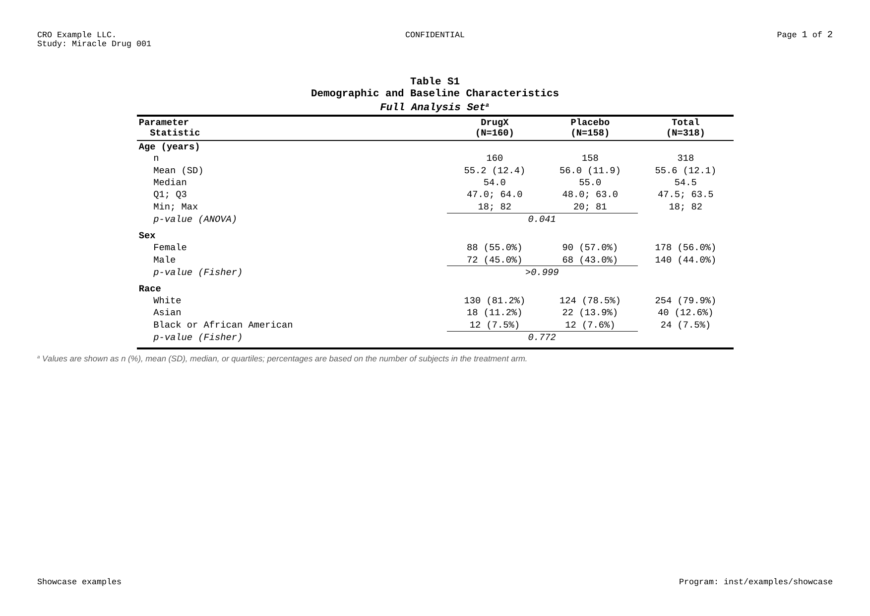
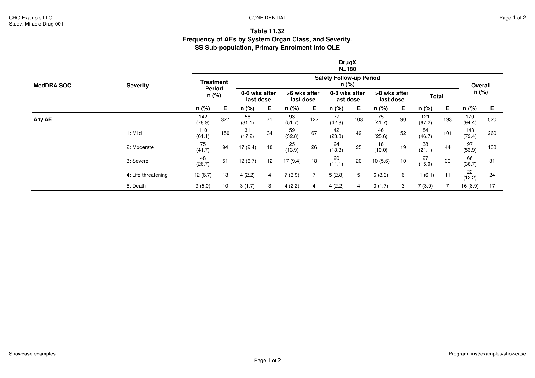
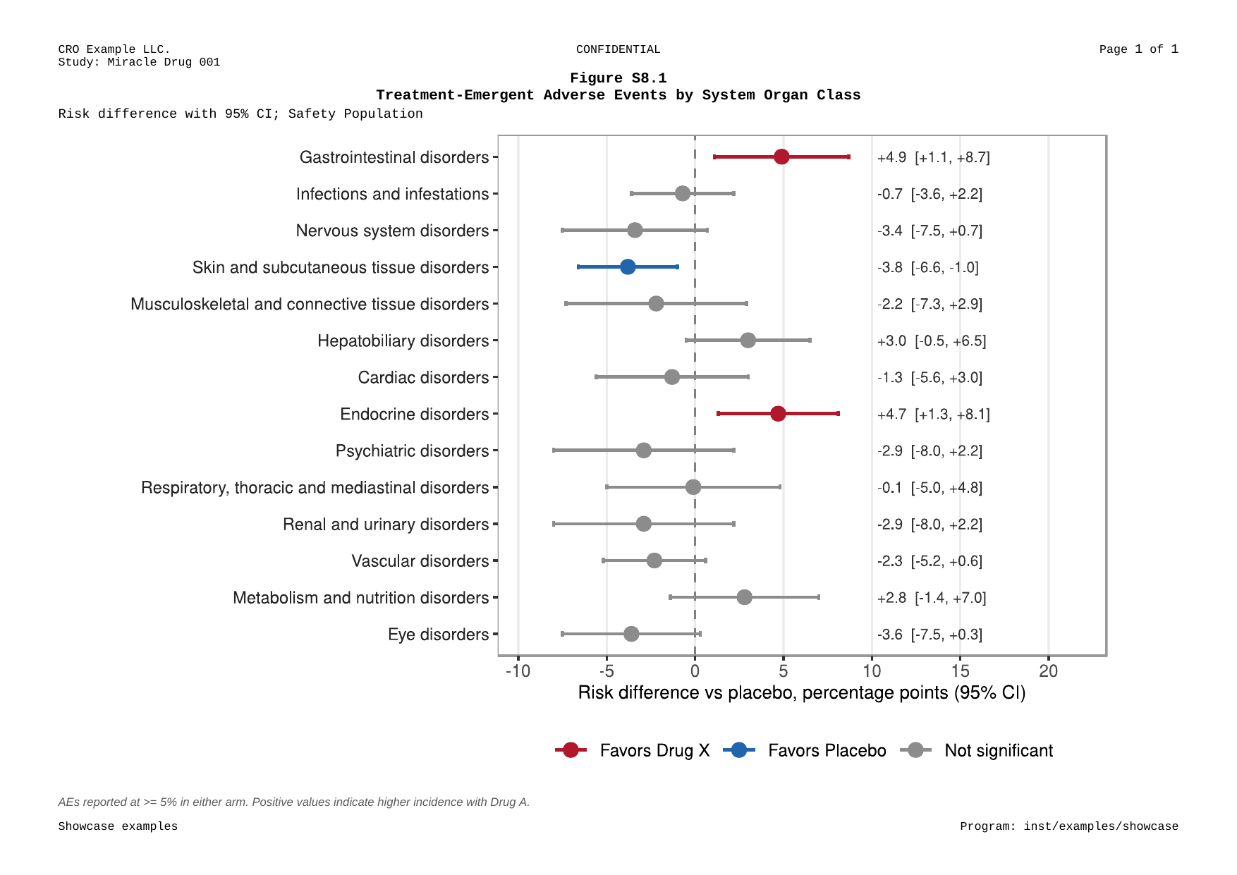
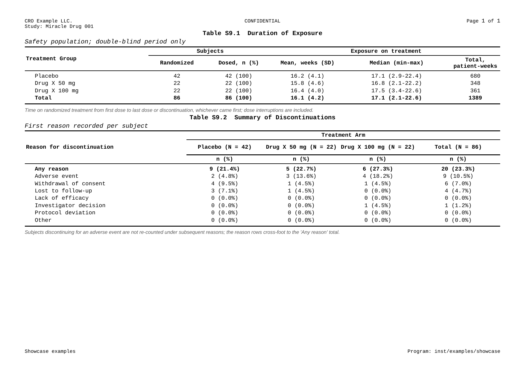
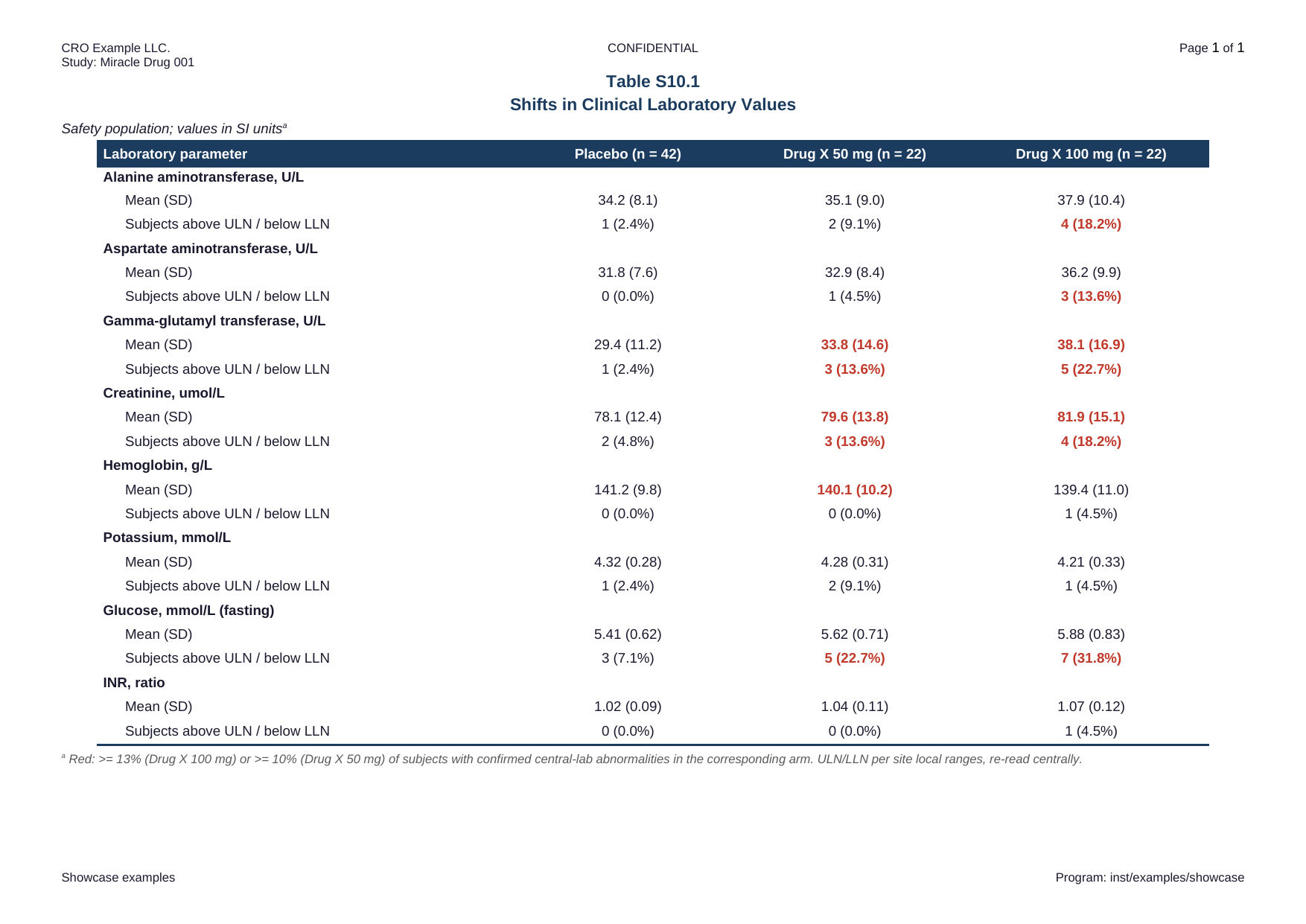
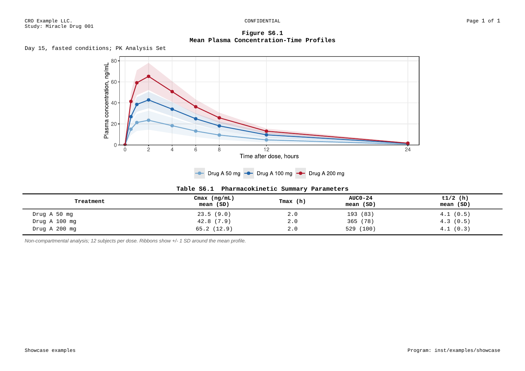
No external tools, no Word macros, no “final_v7_reallyfinal.docx”. One table, one figure, one listing — or all of them, dozens per run, assembled into a single report whose clickable table of contents writes itself. And the endless argument with Word over pagination simply ends: pages break where your spec says they should break, not where Word decides to, so the layout you validated today is the layout on screen a year from now. Every page below was rendered by ksTFL itself. Click a page to open it full size; click its caption to jump to the example walked through line by line in Real Examples.

Demography table with grouped treatment-arm headers — Demography table: grouped headers, merged p-value cells, section rules

Adverse events by system organ class with three-tier spanning headers — Adverse events: three-tier spanning headers, landscape fit

Risk difference forest plot across organ classes — Risk-difference forest plot filling a landscape page

Two summary tables on one page — Exposure and discontinuation tables flowing together on one page

Laboratory table with conditionally colored values — Laboratory safety on the navy template — thresholds highlight themselves

Concentration-time figure with a parameter table — A concentration-time profile and its parameter table as one page

Quick start

This script is all it takes — and yes, iris really is enough:

library(ksTFL)

# any messy source becomes one tidy summary frame - your usual R, nothing exotic
summary <- do.call(rbind, lapply(split(iris, iris$Species), function(g)
  data.frame(Species = g$Species[1], N = nrow(g),
             SL_mean = mean(g$Sepal.Length), SL_sd = sd(g$Sepal.Length),
             PL_mean = mean(g$Petal.Length), PL_sd = sd(g$Petal.Length))))

spec <- create_table(summary) |>
  add_span_header(c(SL_mean, SL_sd), "Sepal", stubOrder = 1) |>
  add_span_header(c(PL_mean, PL_sd), "Petal", stubOrder = 1) |>
  define_cols(c(SL_mean, PL_mean),
              label = c("mean", "mean"), valueStyleRef = "ar", format = "%.2f") |>
  compute_cols(PL_mean < 2.5,
               c_style(c(PL_mean, PL_sd), styleRef = f_combine("fc_green", "b"))) |>
  add_title("Iris, Measured Flower by Flower", styleRef = "b") |>
  add_subtitle("Mean separation of the three species", styleRef = "i") |>
  add_header("Fisher Herbarium", "IRIS STUDY", "Page {PAGE} of {NUMPAGES}") |>
  add_footer("Collected 1936", "", format(Sys.Date(), "Compiled %Y-%m-%d")) |>
  add_footnote("Fisher (1936). Green: petals so distinct the species almost name themselves.") |>
  set_document(contentWidth = "70%")

write_doc(create_report(spec), name = "iris_summary")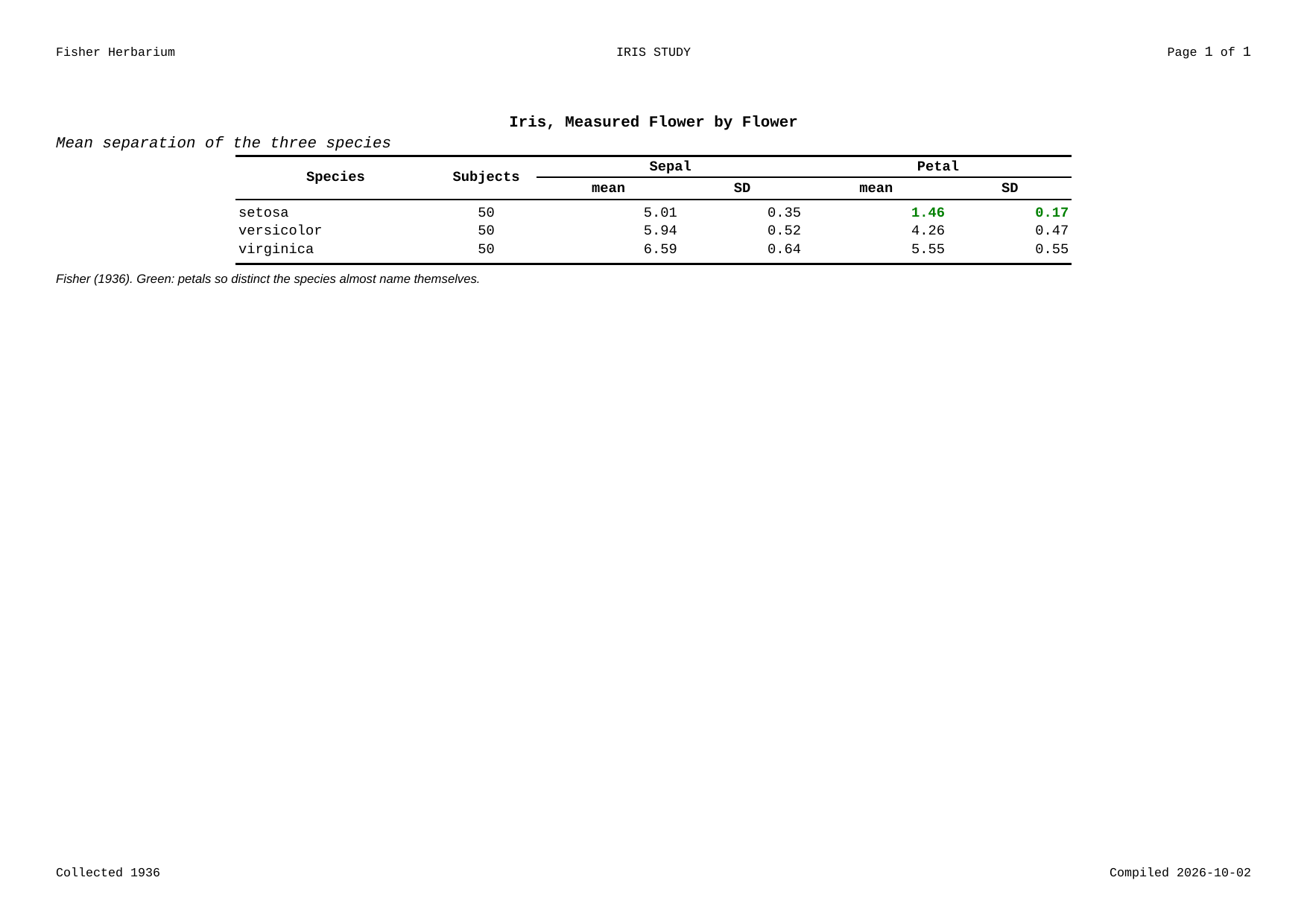

That’s a print-ready Word document — but look at what those lines actually did:

add_span_header() grouped the columns under Sepal and Petal banners, each stretched over its own mean / SD pair. This is the header lattice reviewers expect in a real report — and you declared it in two lines instead of merging cells by hand in Word. Pass the same stubOrder to siblings and a higher one to the umbrella above them: the geometry is your call, the drawing is ksTFL’s.
define_cols() set the look of whole column families at once — valueStyleRef = "ar" right-aligns both means, format = "%.2f" pins every number to two decimals. The style rides with the definition, so it survives whatever the data become next quarter; no per-cell babysitting.
compute_cols() is where it gets fun: “when PL_mean < 2.5, apply c_style() with the fc_green + b atoms” is not an edit, it is a rule. Setosa’s petals turn green now, and every future run re-dyes them automatically — thresholds, colors, and groups stay in the code where they can be reviewed, not lost in a Word session nobody remembers. The style itself is snapped together from built-in atoms via f_combine(): over 120 ready-made pieces (fonts, colors, indents, borders), zero custom style boilerplate.
add_title() / add_subtitle() / add_header() / add_footer() wrote the document’s paperwork — including a live Page {PAGE} of {NUMPAGES} counter that updates itself when the report re-paginates. What you see in the screenshot’s top and bottom bands is exactly the three-slot header/footer API, no Word section wizardry.
set_document(contentWidth = "70%") sized the table to a comfortable reading column, and create_report() + write_doc() did the rest: validation, style consolidation, shaping, pagination — iris_summary.docx lands in your working directory, done.

Run the script, open the file, compare it with the screenshot — that gap between “analysis finished” and “report ready” you’ve been living with? Just closed.

Installation

ksTFL ships pre-compiled binaries for R 4.5 and R 4.6 on Windows, Ubuntu/Debian, Fedora/RHEL, and macOS (ARM) — no compilers or system libraries needed for most users.

The simplest method, works on every platform:

install.packages("ksTFL",
  repos = c("https://crow16384.r-universe.dev", "https://cloud.r-project.org"))

Windows binaries are also available directly:

install.packages("ksTFL",
  repos = "https://crow16384.github.io/ksTFL-release",
  type  = "binary")

Or download finished packages (.zip, .tar.gz, .tgz) from the release repository and install with install.packages(file, repos = NULL).

Building from source requires a C++20 compiler and R development tools (Rtools on Windows, Xcode Command Line Tools on macOS, build-essential on Linux):

remotes::install_github("crow16384/ksTFL")

What else it can do

One look for the whole company. Corporate layouts come built in — pick a template and every table, figure and listing in the run instantly wears the same face: same fonts, same margins, same navy header. Hand a client a submission where nothing drifts from page to page.
It writes around your missing fonts. The package reads the fonts on your machine and quietly substitutes a metric-compatible open-source one when a proprietary font (Arial, Times New Roman, …) isn’t there. The report lays out the same whether you ran it on your laptop or on a Linux build server.
A report that re-builds itself. Every output saves its specification, so you can regenerate the exact same Word document months later, on another machine, without touching the original analysis. Auditors love this; so do you, at 2 a.m. before a submission.
Highlight what matters, by rule. Color a cell red when a value crosses a threshold, bold the first row of every group, drop a section header where the category changes — described once, applied forever, never by hand in Word.
Rich text inside cells. Bold, italic, superscripts, subscripts and line breaks right in your values and titles (H<sub>2</sub>O, p<0.05<sup>*</sup>), the way the final document needs them.
Point and click, if you like. RStudio add-ins give you a template editor and a style picker, so you can compose layouts visually instead of memorizing option names.
Any language, all at once. Cyrillic, CJK, Greek letters and ordinary text share a page without turning into boxes.

Documentation & resources

I want to…	Go to
Learn the workflow in one sitting	Getting Started
Solve a specific problem	FAQ & Troubleshooting
See real examples, table by table	Real Examples and the examples repository
Fine-tune colors, fonts, borders	Styling Guide
Look up any function	Reference
Print a cheat sheet	Cheatsheet (PDF)
Give a talk	Slides (PDF)