Reporting Examples using ksTFL

ksTFL Team

This vignette presents a realistic progression of reporting examples — from minimal tables/listings/figures/text to a full clinical-style table with multi-level headers, spanning stub columns, multi-line titles/footnotes, reusable styles, and session defaults. All examples use exported ksTFL helpers only; set eval=TRUE locally to run the R chunks.

Category and scope

This is a workflow-first vignette for readers who already know the basic pipeline and want practical patterns they can adapt directly.

Related reading:

• Getting Started for the core pipeline.
• Styling Guide, Advanced StyleRows, and Column Width Management for deeper feature coverage.

Workflow overview

Each example follows the same end-to-end pattern so you can reproduce the full pipeline locally:

• Prepare small, self-contained sample data (run the setup chunk with eval=TRUE).
• Build TFL_spec objects using create_table(), create_figure() or create_text().
• Tune columns and styles via define_cols() and add_style() (use f_combine() to reference combined styles).
• Assemble specs into a TFL_report with create_report() (this consolidates style references and assigns dataRef).
• Render to a DOCX with write_doc() (one-step: saves JSON metadata and produces the final document).

Keep in mind:

• Use named styles (add_style()) and reference them by id; avoid inspecting or mutating internal fields.
• Use print(spec) for concise, user-facing previews rather than reading internals, or use the package add-ins for interactive inspection.
• Use metaPath = tempdir() during examples to avoid writing permanent files while you experiment.

# Sample datasets used by multiple sections (run locally before executing examples)
set.seed(2025)

demog_tbl <- data.frame(
  subject_id = sprintf("S%03d", 1:24),
  age = sample(25:80, 24, TRUE),
  sex = sample(c("M","F"), 24, TRUE),
  trt = sample(c("Placebo","DrugA"), 24, TRUE),
  stringsAsFactors = FALSE
)

vitals_tbl <- data.frame(
  subject_id = rep(demog_tbl$subject_id, each = 2),
  visit = rep(c("Baseline","Week 12"), times = 24),
  sbp = round(rnorm(48, 120, 12)),
  dbp = round(rnorm(48, 75, 8)),
  stringsAsFactors = FALSE
)

labs_tbl <- data.frame(
  subject_id = demog_tbl$subject_id,
  ALT = round(rnorm(24, 28, 9)),
  AST = round(rnorm(24, 26, 8)),
  stringsAsFactors = FALSE
)

# Example plot file (created locally when running the vignette)
# type = "cairo" avoids needing an X11 display (headless-safe for pkgdown/CI)
out_dir <- file.path(tempdir(), "ksTFL-reporting-examples")
dir.create(out_dir, recursive = TRUE, showWarnings = FALSE)

plot_file <- file.path(tempdir(), "example_plot.png")
png(plot_file, width = 600, height = 400, type = "cairo")
plot(demog_tbl$age, vitals_tbl$sbp[1:24], xlab = "Age", ylab = "SBP", main = "Age vs SBP")
dev.off()

## Session-wide package and document settings:
tfl_reset_options()
tfl_set_options(
  add_header(c("CRO Example LLC.", "CONFIDENTIAL", "Page {PAGE} of {NUMPAGES}")),
  add_header("Study: Miracle Drug 001"),
  add_footer(c("Showcase examples", "Program: inst/examples/showcase")),
  output_directory = out_dir,
  footnotePlace = "repeated",
  meta_directory = file.path(out_dir, "meta")
)

1 — Simple minimal table

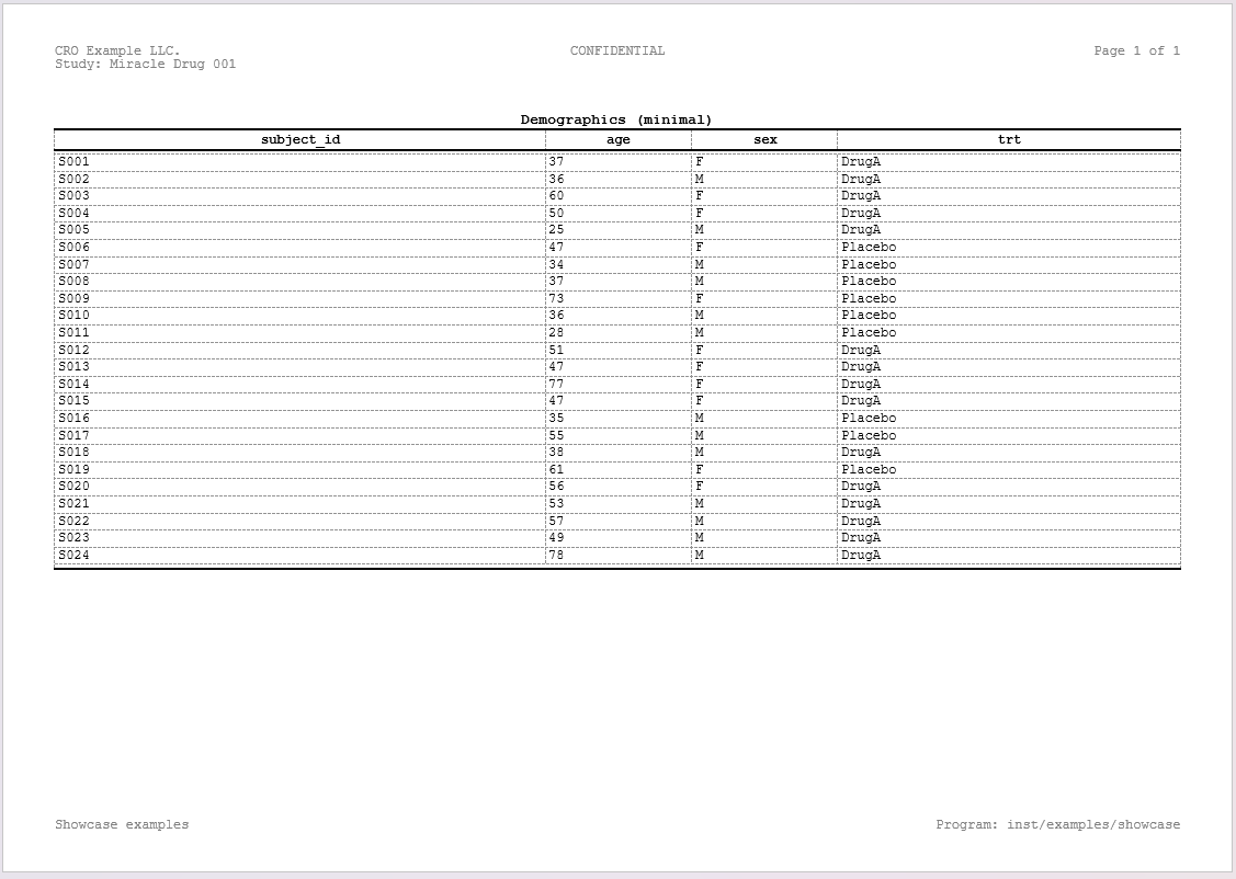
spec_min_table <- create_table(data = demog_tbl, cols = c(subject_id, age, sex, trt))
spec_min_table <- add_title(spec_min_table, "Demographics (minimal)")

# Print shows a compact overview (useful in interactive sessions)
print(spec_min_table)
# close the example chunk

print() on a TFL_spec provides a readable overview including titles and defined columns: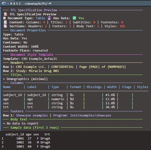

# End-to-end: wrap single spec into a report and render to DOCX
rpt_min_table <- create_report(spec_min_table)
write_doc(rpt_min_table, name = "tbl_min")

Rendered output:

rendered minimal table

A note on the cols parameter — The cols argument in create_table() specifies which columns are rendered in the document and their left-to-right order. It acts purely as a presentation directive: the underlying data frame is stored in full, so columns omitted from cols are not dropped from the spec. They remain available for conditional logic in compute_cols(). For instance, you could exclude a helper column like flag from the report (cols = c(subject_id, age, sex, trt)) yet still reference flag in a compute_cols() condition to drive styling or value transformations. This design means you never need to pre-filter or reorder your data frame before passing it to ksTFL — cols handles column selection and ordering in one place.

2 — Simple minimal figure

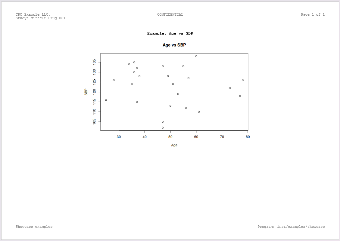
spec_min_fig <- create_figure(plot_file)
spec_min_fig <- add_title(spec_min_fig, "Example: Age vs SBP")
print(spec_min_fig)
# close example chunk

# End-to-end: render the single-figure report to DOCX
rpt_min_fig <- create_report(spec_min_fig)
write_doc(rpt_min_fig, name = "fig_min")

Rendered output:

rendered minimal figure

3 — Simple minimal text (narrative)

## Narrative object:
nartv <- list(
  subj = 'ABC-001',
  enrldt = '01JAN2022',
  compldt = '22JUN2022',
  discreas = 'Completed per protocol',
  nae = 3,
  listae = list('Nausea', 'Vomiting', 'Headache')
)

## Formatted text of the subject narrative:
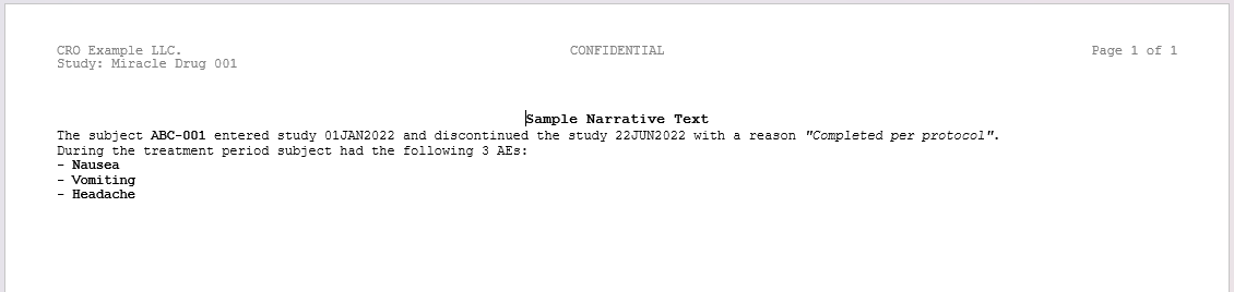
text <- sprintf('The subject <b>%s</b> entered study %s and discontinued the study %s with a reason <i>"%s"</i>.<br>During the treatment period subject had the following %d AEs:<br><b>- %s</b>', 
        nartv[["subj"]],
        nartv[["enrldt"]],
        nartv[["compldt"]],
        nartv[["discreas"]],
        nartv[["nae"]],
        paste(nartv[["listae"]], collapse = '<br>- ')
)

# End-to-end: render the narrative report to DOCX
spec_min_text <- create_text() |> add_title("Sample Narrative Text")
spec_min_text <- add_body_text(spec_min_text, text)
rpt_min_text <- create_report(spec_min_text)
write_doc(rpt_min_text, name = "nar_min")

Rendered output:

rendered narrative text

4 — Define columns: single, batch, and parameter recycling

Why define_cols()?

After creating a table with create_table(), column properties are auto-detected from the data. However, you often need to: - Customize column labels for readability - Specify numeric formats (e.g., “%.2f” for 2 decimal places) - Control visibility, styling, or special behaviors (ID column, deduplicate, page breaks) - Lock or adjust column widths for better layout

define_cols() is the primary tool for these customizations. It supports both single-column and batch updates, with intelligent parameter recycling to keep code concise.

Example 1: Single column definition

The simplest case — modify one column at a time:

# Define one column
spec_single <- create_table(data = demog_tbl, cols = c(subject_id, age, sex, trt))
spec_single <- define_cols(spec_single, subject_id, label = "Subject ID", isID = TRUE)

# Another single column call (chaining is encouraged)
spec_single <- define_cols(spec_single, age, 
                           label = "Age (years)", 
                           type = "numeric", 
                           format = "%.0f")

print(spec_single)
# close example chunk

Example 2: Batch update with single value (recycling to all columns)

Update multiple columns with the same value — the value is automatically recycled:

# Apply single format to multiple columns
spec_batch <- create_table(data = vitals_tbl, cols = c(sbp, dbp))
spec_batch <- define_cols(spec_batch, c(sbp, dbp),
                          type = "numeric",      # Applied to both
                          format = "%.1f",       # Applied to both
                          valueStyleRef = "b")  # Applied to both

print(spec_batch)
# close example chunk

Why this matters: Instead of writing three separate define_cols() calls, you write one line and the package applies the same values to all selected columns.

Example 3: Batch update with per-column values (1-to-N mapping)

Update multiple columns with different values — provide a vector matching the number of columns:

# Different label and format for each column
spec_mapped <- create_table(data = demog_tbl, cols = c(age, sex, trt)) |>
define_cols(c(age, sex, trt),
            label = c("Age (years)", "Biological Sex", "Treatment Group"),
            type = c("numeric", "string", "string"),
            format = c("%.0f", NA, NA) #format not applicable for strings -> NA
)

print(spec_mapped)
# close example chunk

Important: The vector length must match exactly:

- Length 1: applies to all columns

- Length N (where N = number of columns): applies one-to-one

- Any other length: raises an error

Example 4: Multiple define_cols() calls (chaining with |>)

Combine define_cols() calls to layer customizations — each call merges with previous settings (last-win strategy):

# Start with basic table
spec_chain <- 
  create_table(data = demog_tbl, cols = c(subject_id, age, sex, trt)) |>
# First pass: set all labels
  define_cols(c(subject_id, age, sex, trt),
             label = c("Subject ID", "Age", "Sex", "Treatment")) |>
# Second pass: set numeric formatting for age
  define_cols(age, type = "numeric", format = "%.0f") |>
# Third pass: mark subject_id as ID column (repeats on page breaks)
  define_cols(subject_id, isID = TRUE)

print(spec_chain)
# close example chunk

This approach makes it easy to:

- Define labels first (human-readable column names)

- Then apply formatting (numeric/string types, decimals)

- Then apply special behavior flags (ID, deduplicate, etc.)

---

5 — Set document properties (hasData, content width, placement)

Key function: set_document()

• hasData: Whether document contains data (important for Text specs)

- footnotePlace: Control placement of titles, footnotes, and subtitles

- contentWidth: Content width (e.g., “100%”, “6.5in”, “16.51cm”)

- isContinues: Ignore page breaks between sections

Example 1: hasData flag

spec <- create_table(demog_tbl) #automatically detects if dataframe has any rows
# When data frame does not have any rows, the report will show the default body_text placeholder instead of empty table. 
#body text can be manually specified

spec <- set_document(spec,
  hasData = FALSE) #override autodetected value

print(spec)

Example 2: Content width and placement

spec <- create_table(demog_tbl)

spec <- set_document(spec,
  contentWidth = "95%",        # Narrower content (default 100%)
  footnotePlace = "repeated")  # Footnotes on every page

Notes:

- Most defaults are sensible; you typically only need set_document() for content width

- Multiple calls merge with last-win strategy (later calls override earlier ones)

---

6 — Combine table/figure/text into a single report

report_simple <- create_report(spec_min_table, spec_min_fig, spec_min_text)

# Render combined simple report to DOCX
write_doc(report_simple, name = "report_simple")

Notes: create_report() preserves input order and consolidates styles. Additionally, with toc = TRUE parameter the table of contents can be generated [in order this to work the titles in the input specs should be marked for toc entries - see ?add_title]

Passing a named list of specs

When specs are built independently (e.g. in a loop, across separate program files, or inside a function that returns a list), they can be collected into a named list and passed as a single argument:

specs <- list(
  t_dm   = spec_min_table,
  t_fig  = spec_min_fig,
  t_text = spec_min_text
)

# Equivalent to create_report(spec_min_table, spec_min_fig, spec_min_text)
# but the list can be assembled dynamically.
report_from_list <- create_report(specs)

# List names become key prefixes:
# names(report_from_list)
# [1] "t_dm_<hash>"   "t_fig_<hash>"  "t_text_<hash>"

List arguments may be freely mixed with variadic specs and reports:

extra_spec <- create_text() |> add_body_text("Appendix note.")

report_mixed <- create_report(extra_spec, specs)

Unnamed list elements fall back to <outer_arg_name>_<i> (e.g. specs_1, specs_2, …). TFL_report objects inside a list are flattened with their original keys preserved.

---

7 — Column widths: automatic calculation and locking

How automatic column width works

When you create a table with create_table(), ksTFL automatically analyzes the data and distributes column widths proportionally:

1. Initial analysis: For each column, the package examines data values (length, type, number of decimals)
2. Width calculation: Numeric columns typically get wider if they have many decimals or large values; short text columns get narrower
3. Proportional distribution: All widths are normalized to sum to 100% (or remaining available width)
4. Default: autoColWidth = TRUE in package options (can be changed with tfl_set_options())

Example: A table with columns id (short numeric), description (long text), value (numeric): - Auto-detected widths might be: id = 20%, description = 50%, value = 30%

Example 1: Accept auto-calculated widths

The simplest approach — let the package handle width distribution:

# Create table; widths are auto-calculated from data characteristics
spec_auto <- create_table(data = labs_tbl, cols = c(subject_id, ALT, AST))
spec_auto <- define_cols(spec_auto, c(subject_id, ALT, AST),
                         label = c("Subject ID", "ALT (U/L)", "AST (U/L)"))

# Print to see auto-calculated widths
print(spec_auto)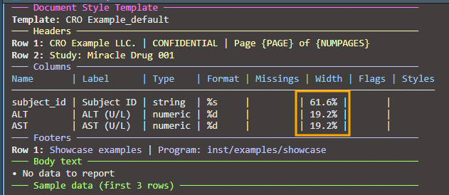

colwidth auto calculated

Example 2: Lock one column, auto-adjust others

Lock a specific column width while others recalculate to fill remaining space:

# Lock subject_id at 15%, let ALT and AST split the remaining 85%
spec_lock1 <- create_table(data = labs_tbl, cols = c(subject_id, ALT, AST))
spec_lock1 <- define_cols(spec_lock1, subject_id, 
                          label = "Subject ID",
                          colWidth = "15%")  # Lock at 15%

# When auto-recalculation runs (automatic), ALT and AST widths are recalculated
# to maintain their initial proportion while filling the remaining 85%

print(spec_lock1)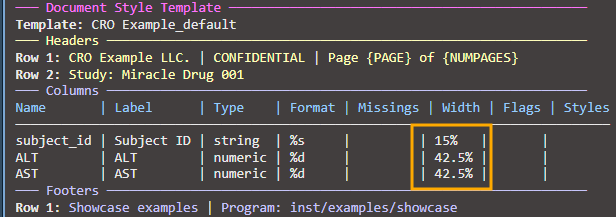

colwidth single locked

Example 3: Lock multiple columns with relative widths

Lock several columns and let others auto-adjust:

# Lock two columns, let the third auto-adjust
spec_lock_multi <- create_table(data = labs_tbl, cols = c(subject_id, ALT, AST))
spec_lock_multi <- define_cols(spec_lock_multi, subject_id, 
                               label = "Subject ID",
                               colWidth = "12%")
spec_lock_multi <- define_cols(spec_lock_multi, ALT,
                               label = "ALT (U/L)",
                               colWidth = "40%")

# AST automatically fills remaining 48% (100% - 12% - 40%)

print(spec_lock_multi)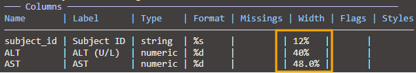

colwidth multiple locked

Example 4: Mixed units (percentages and absolute)

Combine percentage-based widths with absolute units:

# Lock subject_id at 2 cm, others in percentages
spec_mixed <- create_table(data = labs_tbl, cols = c(subject_id, ALT, AST))
spec_mixed <- define_cols(spec_mixed, subject_id,
                          label = "Subject ID",
                          colWidth = "2cm")  # Absolute width
spec_mixed <- define_cols(spec_mixed, ALT,
                          label = "ALT (U/L)",
                          colWidth = "35%")   # Percentage of remaining

print(spec_mixed)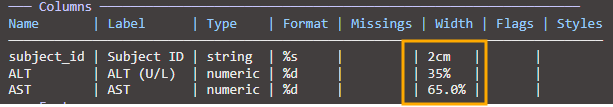

colwidth mixed units

Important: When mixing units (cm, in, pt) with percentages, the absolute widths are reserved first, then percentages are calculated from remaining space.

Example 5: Width validation and constraints

The package validates column widths to prevent invalid configurations:

spec_valid <- create_table(data = labs_tbl, cols = c(subject_id, ALT, AST))

# VALID: Set a reasonable relative width
spec_valid <- define_cols(spec_valid, ALT,
                          colWidth = "30%")  # OK: 30% is valid

# INVALID: Cannot set 100% relative width (leaves no space for other columns)
# This will raise an error:
# spec_valid <- define_cols(spec_valid, ALT, colWidth = "100%")
# Error: relative width 100.0% exceeds maximum allowed 75.0% 
#        (accounting for locked columns and minimum 0.5% for other columns)

# INVALID: Cannot set width below minimum threshold
# spec_valid <- define_cols(spec_valid, AST, colWidth = "0.2%")
# Error: relative width 0.2% is below minimum 0.5%

# Minimum width constraints (can be customized via package options):
# - Relative widths (%): minimum 0.5%
# - Fixed widths (cm, in, pt): minimum 0.2cm (~2mm, ~0.08in)

# Configure minimum width via package options:
tfl_set_options(minColWidth = 1.0)  # Set minimum relative width to 1.0%

# Now 0.5% will fail, but 1.0% will succeed
spec_valid <- define_cols(spec_valid, AST,
                          colWidth = "1.0%")  # OK with new minimum

print(spec_valid)

Width validation rules:

- Relative width (%): Must be ≥ minColWidth (default 0.5%)

- Relative width (%): Cannot exceed max allowed considering locked columns and other column minimums

- Fixed width: Must be ≥ 0.2cm (all units: cm, in, pt, mm automatically converted)

- Incompatible widths: Cannot set width to 100% (would exclude all other columns)

Error messages are detailed and show the maximum allowed width when you exceed limits:

Error: relative width 100.0% exceeds maximum allowed 75.0% 
       (accounting for 2 locked columns requiring 25% total, 
        and minimum 0.5% for remaining 1 unlocked column)

---

8 — Table with titles, subtitles and footnotes

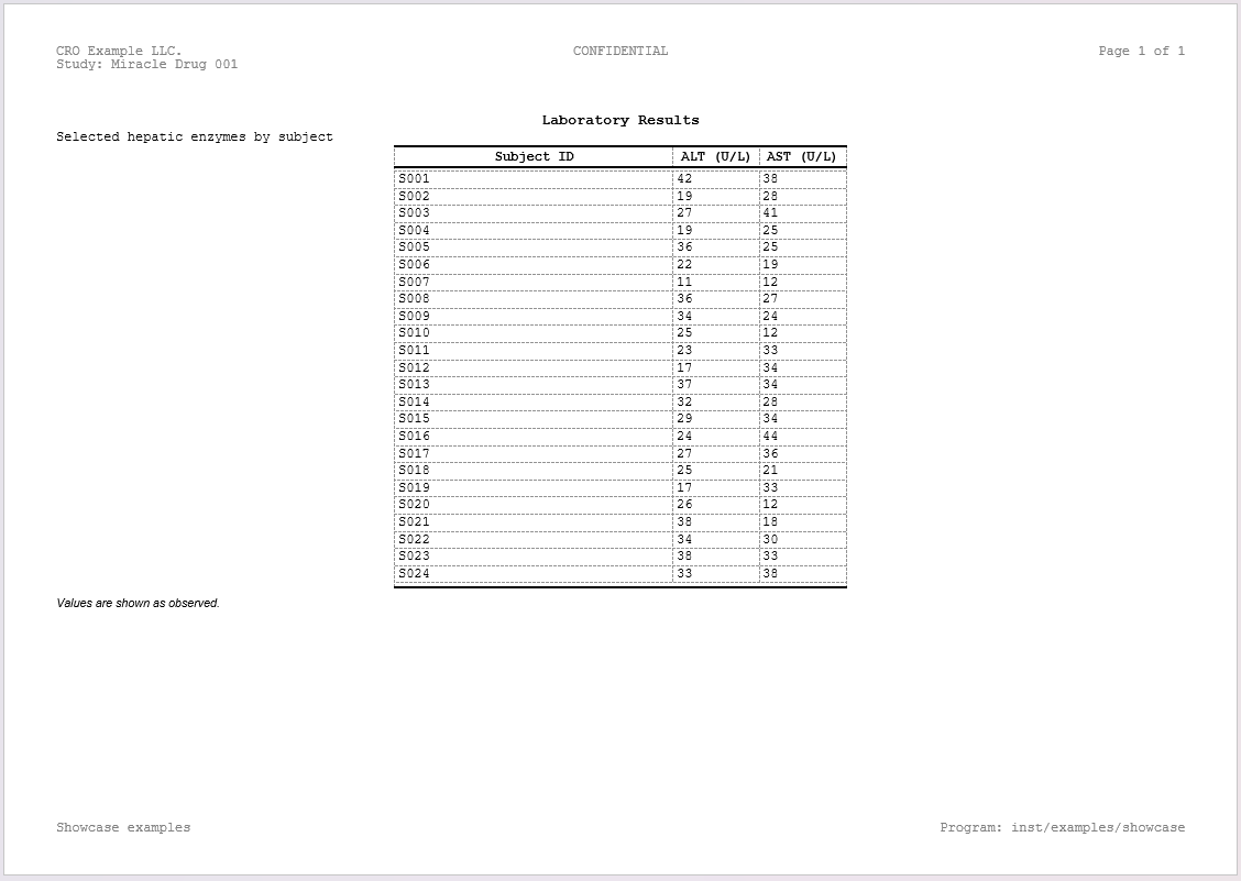
spec_multi <- create_table(data = labs_tbl, cols = c(subject_id, ALT, AST))
spec_multi <- add_title(spec_multi, "Laboratory Results")
spec_multi <- add_subtitle(spec_multi, "Selected hepatic enzymes by subject")
spec_multi <- add_footnote(spec_multi, "Values are shown as observed.")

spec_multi <- define_cols(
  spec_multi,
  c(subject_id, ALT, AST),
  label = c("Subject ID", "ALT (U/L)", "AST (U/L)")
)

print(spec_multi)
# close example chunk

# Render the multilevel table to DOCX
rpt_multi <- create_report(spec_multi)
write_doc(rpt_multi, name = "tbl_multi")

Rendered output:

table titles subtitles footnotes

9 — span columns (spanning headers)

Why spanning headers?

In clinical tables, you often need to group related columns under a common header. For example: - “Baseline” spanning columns: visit, sbp, dbp, pulse - “Week 12” spanning columns: sbp, dbp, pulse (repeated measurements at different visits)

Spanning headers (called “spans” in ksTFL) are separate from column labels — they sit above the column labels and group multiple columns. Multiple spans can be stacked at different vertical levels.

Example 1: Single spanning header

Create one stub that groups related columns:

# Start with demographics table
spec_span_simple <- create_table(data = demog_tbl, cols = c(subject_id, age, sex, trt))
spec_span_simple <- define_cols(spec_span_simple, 
                                c(subject_id, age, sex, trt), 
                                label = c("Subject","Age","Sex","Treatment"))

# Add a spanning header for "Demographics" above age and sex
spec_span_simple <- add_span_header(spec_span_simple, 
                                    cols = c("age", "sex"), 
                                    label = "Demographics")

print(spec_span_simple)

Result: A table with column labels on one row and a “Demographics” header spanning age+sex columns above it: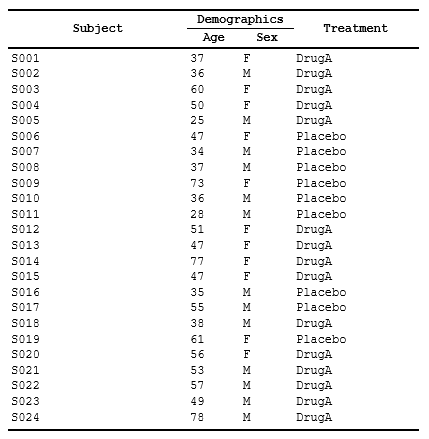

Example 1b: Using tidyselect helpers with spanning headers

add_span_header() supports all tidyselect expressions — use helpers for flexible column selection:

# Table with mixed column types
mixed_data <- data.frame(
  id = 1:10,
  age_baseline = rnorm(10, 45, 10),
  age_follow = rnorm(10, 46, 10),
  weight_baseline = rnorm(10, 70, 10),
  weight_follow = rnorm(10, 71, 10)
)

spec_tidysel <- create_table(mixed_data)

# Using starts_with() helper
spec_tidysel <- add_span_header(spec_tidysel, 
                                cols = starts_with("age"),
                                label = "Age Measurements",
                                stubOrder = 1) |>
# Using col position 
add_span_header(cols = c(4,5),
               label = "Weight Measurements",
               stubOrder = 1) |>
# Using negation (-) to exclude columns
add_span_header(cols = -id,
                label = "Baseline and Follow",
                stubOrder = 2)

print(spec_tidysel)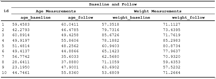

span header tidyselect

Tidyselect expressions supported:

- Ranges: cols = age:weight (all columns between age and weight)

- Helpers: cols = starts_with("age"), contains("baseline"), matches("^w")

- Negation: cols = -id (all columns except id)

- Combinations: cols = c(starts_with("age"), weight_baseline)

Example 2: Styled spanning headers

Apply styles to stub labels using labelStyleRef:

# First, create a style for stub labels
spec_spans_style <- create_table(data = demog_tbl, cols = c(subject_id, age, sex, trt))

spec_spans_style <- add_style(spec_spans_style, 
                              id = "span_header",
                              s_font(bold = TRUE, font_size = "12pt"),
                              s_paragraph(alignment = "center"),
                              s_table_style(background_color = "#E8E8E8"))

# Define columns
spec_spans_style <- define_cols(spec_spans_style,
                                c(subject_id, age, sex, trt),
                                label = c("Subject ID", "Age", "Sex", "Treatment"),
                                valueStyleRef = 'ac')

# Add span with style reference
spec_spans_style <- add_span_header(spec_spans_style,
                                    cols = c("age", "sex"),
                                    label = "Demographics",
                                    labelStyleRef = "span_header")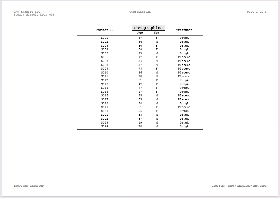

span header styled

Notes:

- labelStyleRef can be a single style name or multiple styles combined with f_combine()

- Span labels inherit the applied style, making grouped columns visually distinct

- Styles must be defined before referencing them in add_span_header()

Example 3: Paragraph borders on spanning headers

When a cell border is applied to a spanning header, it stretches across the entire merged cell. A paragraph border instead follows the text width — useful for visually separating groups without a full-width line. Paragraph borders are also unaffected by structural border overrides (header_top_border, header_bottom_border), giving full control on intermediate header rows.

spec_para <- create_table(data = demog_tbl, cols = c(subject_id, age, sex, trt))

# Paragraph border style — the underline follows the text, not the cell edge
spec_para <- add_style(spec_para, id = "span_underline",
  s_font(bold = TRUE),
  s_paragraph(
    alignment = "center",
    borders = s_borders(
      bottom = s_border(color = "#000000", width = "0.5pt", line_style = "single")
    )
  )
)

# Or use the built-in paragraph border atom
spec_para <- add_span_header(spec_para,
  cols = c("age", "sex"),
  label = "Demographics",
  labelStyleRef = f_combine("b", "ac", "pb_th")  # bold + center + thin paragraph bottom border
)

# Render stubbed table report to DOCX
rpt_stub <- create_report(spec_stubs_style)
write_doc(rpt_stub, name = "tbl_stub", outDir = "./out", metaPath = tempdir())

---

10 — Styles and f_combine() for combined style references

Why named styles?

Styles are foundational in professional reporting:

- Define once, reference many times — consistency across your document

- Easy to update: change one style definition and all references automatically pick up the change

- Composable: combine base styles (bold, red text) into complex styles for specific use cases

ksTFL uses a named style system: you define styles with add_style() giving each an id, then reference them by name wherever you need them (labelStyleRef, valueStyleRef, labelStyleRef in stubs, etc.).

Example 1: Define base styles

Create atomic styles that focus on one aspect (font, alignment, color):

# Create a table spec
spec_base_styles <- create_table(data = demog_tbl, cols = c(subject_id, age, sex, trt))

# Define reusable base styles
spec_base_styles <- add_style(spec_base_styles, id = "bold_header",
                              s_font(bold = TRUE, font_size = "12pt"))

spec_base_styles <- add_style(spec_base_styles, id = "right_align",
                              s_paragraph(alignment = "right"))

spec_base_styles <- add_style(spec_base_styles, id = "light_gray_bg",
                              s_table_style(background_color = "#F5F5F5"))

# Apply to columns
spec_base_styles <- define_cols(spec_base_styles,
                                c(subject_id, age, sex, trt),
                                label = c("Subject ID", "Age", "Sex", "Treatment"),
                                labelStyleRef = c("bold_header", "", "", ""))

print(spec_base_styles)
# close example chunk

Example 2: Combine styles with f_combine()

Apply multiple styles to a single element using f_combine() — they merge at render time:

# Create spec and define base styles
spec_combined <- create_table(data = demog_tbl, cols = c(subject_id, age, sex, trt))

# Define atomic styles
spec_combined <- add_style(spec_combined, id = "bold_text", s_font(bold = TRUE))
spec_combined <- add_style(spec_combined, id = "red_color", s_font(color = "#CC0000"))
spec_combined <- add_style(spec_combined, id = "centered", s_paragraph(alignment = "center"))

# Combine styles: bold + red text + centered
spec_combined <- define_cols(spec_combined,
                             subject_id,
                             label = "Subject ID",
                             labelStyleRef = f_combine("bold_text", "red_color", "centered")) |>

define_cols(c(sex, trt),
            label=c('Sex', 'Treatment'),
            labelStyleRef = f_combine('b','i'),
            valueStyleRef = f_combine('ar', 'i')
            ) |>
# Different columns can use different combinations
define_cols(age, label = "Age",
            labelStyleRef = f_combine("bold_text", "centered"),
            valueStyleRef = 'ac')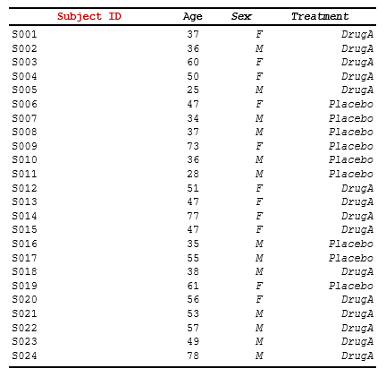

styles fcombine columns

How f_combine() works:

- Takes multiple style names as arguments

- Returns a reference object that tells the package to merge those styles

- Order matters for last-win conflict resolution (later arguments override earlier ones)

11 — Conditional row actions with compute_cols()

Overview: While define_cols() sets properties globally for all rows, compute_cols() applies conditional actions to specific rows matching a condition.

Common use cases:

- Style rows where a specific value occurs (e.g., first/last occurrence, threshold-based)

- Merge columns in certain rows (e.g., group headers)

- Insert separator or summary rows programmatically

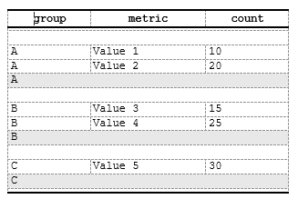
Example 1: Conditional styling

Apply a style to columns in rows matching a condition:

# Sample data with groups
data <- data.frame(
  group = c("A", "A", "B", "B", "C"),
  metric = c("Value 1", "Value 2", "Value 3", "Value 4", "Value 5"),
  count = c(10, 20, 15, 25, 30)
)

# Create spec and define styles
spec <- create_table(data) |>
  add_style(id = "group_header", s_font(bold = TRUE, color = "#0000FF")) |>
  add_style(id = "emphasize",    s_table_style(background_color = "#FFFFCC"))

# Apply conditional styling: bold+blue for first occurrence of each group
spec <- spec |>
  compute_cols(firstOf(group), c_style(c(metric, count), styleRef = "group_header"))

# Apply conditional styling: highlight rows with high count
spec <- spec |>
  compute_cols(count > 20, c_style(count, styleRef = "emphasize"))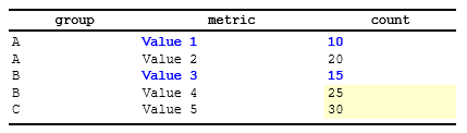

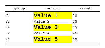
compute conditional styling

Example 2: Combining styles in conditional rows

Apply multiple styles to a single column using f_combine():

spec <- create_table(data) |>
  add_style(id = "bold",      s_font(bold = TRUE)) |>
  add_style(id = "large",     s_font(font_size = "14pt")) |>
  add_style(id = "highlight", s_table_style(background_color = "#FFFF00"))

# Apply combined styles to first group occurrence
spec <- spec |>
  compute_cols(firstOf(group), 
    c_style(metric, styleRef = f_combine("bold", "large", "highlight"))
  )

compute combined styles

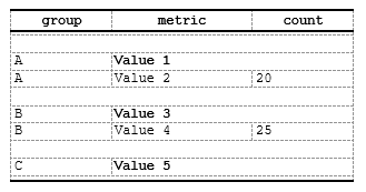
Example 3: Column merging in conditional rows

Merge adjacent columns for rows matching a condition:

spec <- create_table(data) |>
  add_style(id = "group_label", s_table_style(background_color = "#D9D9D9"))

# Merge metric and count columns for first occurrence (group header style)
spec <- spec |>
  compute_cols(firstOf(group), 
    c_merge(c(metric, count), styleRef = "group_label")
  )

compute column merging

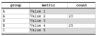
Example 4: Inserting separator rows

Insert empty rows (separators) or rows with content from another column:

spec <- create_table(data) |>
  add_style(id = "separator", s_table_style(background_color = "#E8E8E8"))

# Insert empty separator above first group occurrence
spec <- spec |>
  compute_cols(firstOf(group), 
    c_addrow(pos = "above")  # Empty row, no value_from
  )

# Insert summary row below last group occurrence (using a specific column as content)
spec <- spec |>
  compute_cols(lastOf(group), 
    c_addrow(pos = "below", value_from = "group", styleRef = "separator")
  )

compute row insertion

Example 4b: Page break insertion

Force a page break when a group ends (useful for long groups):

spec <- spec |>
  compute_cols(lastOf(group),
    c_pageBreak()
  )

Example 5: Multiple actions on same rows

Combine styling, merging, and row insertion in a single compute_cols() call:

spec <- create_table(data) |>
  add_style(id = "header",    s_font(bold = TRUE)) |>
  add_style(id = "separator", s_table_style(background_color = "#E8E8E8"))

# For first group occurrence: add separator, style, and merge
spec <- spec |>
  compute_cols(firstOf(group), 
    c_addrow(pos = "above"),  # Add empty separator
    c_style(metric, styleRef = "header"),  # Style metric column
    c_merge(c(metric, count))  # Merge adjacent columns
  )

compute multiple actions

Key concepts:

- Conditions are unevaluated expressions evaluated at report generation time (during create_report())

- Helper functions (firstOf(), lastOf(), firstRow(), lastRow(), rowNumber(), everyNth(), firstOfBlock()) are only available inside compute_cols() conditions — they are not standalone exported functions. See vignette("Advanced_StyleRows") for full details.

- Multiple calls accumulate: calling compute_cols() multiple times on the same spec appends actions

- Multiple actions in one call: same row can have styling, merging, and row insertion simultaneously

- Overlapping conditions: if multiple conditions match the same row, all actions apply (styling aggregates, merging rules apply) - value_from: Optional in c_addrow() — omit for empty separator rows

- Performance: Conditions evaluated once per row during report assembly; style consolidation happens automatically

---

12 — Render to DOCX with write_doc()

What write_doc() does

write_doc() is the primary output function. It combines two lower-level steps into one:

1. Validates and serializes the report to JSON, writing metadata and data files to metaPath
2. Renders the JSON to a DOCX file in outDir

create_report() → write_doc()  →  output.docx

Example: Assemble and render a multi-spec report

Tip: Use tfl_list_templates() to discover available template names (e.g., "Navy_Pro", "Carbon_Dark"). Use run_styles_editor() to interactively preview and customize templates.

# Create multiple specs
table_spec <- create_table(data = labs_tbl, cols = c(subject_id, ALT, AST))
table_spec <- add_title(table_spec, "Laboratory Results")
table_spec <- set_page_style(table_spec, docTemplate = "Navy_Pro")

text_spec <- create_text()
text_spec <- add_body_text(text_spec, "All values are from the locked database.")
text_spec <- set_page_style(text_spec, docTemplate = "Carbon_Dark")

# Assemble into report
report_full <- create_report(table_spec, text_spec)

# A) Per-spec templates (default): each spec uses its own docTemplate
write_doc(report_full, name = "example_report", outDir = "./out", metaPath = tempdir())

# B) Global override: force one template for all specs
write_doc(
  report_full,
  name = "example_report_global_override",
  outDir = "./out",
  metaPath = tempdir(),
  overrideTemplate = system.file("templates", "Navy_Pro.json", package = "ksTFL", mustWork = TRUE)
)

In this workflow:

• write_doc(..., overrideTemplate = NULL) keeps per-spec docTemplate styling.
• write_doc(..., overrideTemplate = <name_or_path>) applies a single global template to all specs.

Key parameters:

• report: A TFL_report object created via create_report().
• name: Base name for the output DOCX ("example_report" becomes example_report.docx).
• outDir: Directory where the output DOCX is written.
• metaPath: Directory where intermediate JSON and data files are written.

Advanced: If you need to inspect the JSON before rendering (e.g. for debugging or CI pipelines), you can split the call into save_report() + replay_report(). See ?write_doc and ?replay_report for details.

---

13 — Session-wide tfl_options: common headers/footers and default body text

Why session options?

In a real clinical reporting workflow, many tables/listings share: - Common headers (study name, database version, confidentiality notice) - Common footers (company name, page numbers, disclaimers) - Default body text (standard disclaimers or methodology notes)

Instead of adding these to every spec, use tfl_set_options() to set session defaults once. All specs created afterward inherit these settings.

Example 1: Set basic session options

# Set session defaults (applies to all NEW specs created after this call)
tfl_set_options(
  add_header("Study ABC", "Phase II Safety Study", "CONFIDENTIAL"),
  add_footer("Company Confidential", "Page {PAGE} of {NUMPAGES}")
)

# Create spec — automatically inherits headers/footers from options
spec_with_opts <- create_table(data = demog_tbl, cols = c(subject_id, age, sex, trt))
spec_with_opts <- add_title(spec_with_opts, "Demographics Table")

print(spec_with_opts)
# close example chunk

Key point: Headers and footers from tfl_set_options() are automatically applied to new specs. No need to call add_header() again.

Example 2: Override session options in a specific spec

You can override session defaults on individual specs:

# Session options are still in effect from previous example

# Create a spec with session defaults
spec_default <- create_table(data = labs_tbl, cols = c(subject_id, ALT, AST))
spec_default <- add_title(spec_default, "Lab Results (using session defaults)")

# Create another spec but override the header
spec_override <- create_table(data = demog_tbl, cols = c(subject_id, age))
spec_override <- add_header(spec_override, "Study XYZ", "Different Study", "CONFIDENTIAL")  # Overrides session default
spec_override <- add_title(spec_override, "Demographics (custom header)")

print(spec_default)   # Uses session header from tfl_set_options
print(spec_override)  # Uses custom header from add_header call
# close example chunk

Rule: Spec-level settings always take precedence over session defaults (last-win strategy).

Example 3: Check and reset session options

Inspect current session options and reset to defaults:

# Check current options
current_options <- tfl_get_options()
str(current_options)

# Get a single option
current_missings <- tfl_get_option("missings")
cat("Current missings representation:", current_missings, "\n")

# Reset to package defaults
tfl_reset_options()

# Now new specs will use package defaults instead of your custom session options
spec_reset <- create_table(data = demog_tbl, cols = c(subject_id, age))
print(spec_reset)
# close example chunk

---

Final notes

This vignette stays deliberately example-heavy. Reuse it when you want a compact pattern for a minimal spec, a multi-spec report, span headers, width tuning, or session-level defaults.

Running examples locally: Set the top chunk eval=TRUE to generate sample data, then execute examples in order. All code uses exported functions only — no internal API manipulation needed.

For more details on function parameters, see the roxygen documentation: ?create_table, ?define_cols, ?add_style, ?write_doc, etc.