Getting Started with ksTFL

Introduction

What is ksTFL?

ksTFL is a lightweight R toolkit for building metadata specifications for clinical Tables, Figures, and Text (TFLs). Unlike traditional table formatters (flextable, huxtable, officer), ksTFL separates metadata generation from rendering:

You define the document structure, content, column formats, and styles in R.
ksTFL generates a structured specification (JSON metadata + data files).
The built-in C++ renderer turns it into a DOCX document with deterministic HarfBuzz-based pagination, via write_doc() or replay_report().

The split pays off in four ways: every table follows the same style templates, 50+ tables can be generated from one program with minimal code, specifications are version-controllable and auditable, and the renderer is separable from the R code that builds the spec.

Reach for ksTFL when you need:

Regulatory clinical reporting (FDA, EMA submissions).
Large-scale automated reporting (100+ tables from common data sources).
Complex table structures: multi-level headers, spanning columns, conditional formatting.
JSON metadata artifacts for downstream processing.

How to use this guide

This is the foundation vignette and the starting point for new users: core objects, main function flow, and the smallest complete pipeline.

Reading order after this vignette:

Reporting Examples and FAQ for the quickest practical follow-up.
Styling Guide, Column Width Management, and Advanced StyleRows for focused feature depth.
Real Examples for fuller clinical-style outputs, then Font Management and Rendering Pipeline when you need environment or renderer internals.

General workflow

High-level pipeline

Data Frame / Image File
       ↓
create_table() / create_figure() / create_text()
       ↓
TFL_spec (customize with define_cols(), add_style(), add_span_header(),
         add_title(), compute_cols(), set_page_style(), set_document())
       ↓
create_report() (assemble specs, consolidate styles)
       ↓
TFL_report
       ↓
write_doc() ────────────────→ Styled .docx
save_report() → replay_report() ─┘  (two-step: inspect JSON first)
(C++ engine, deterministic HarfBuzz pagination)

Anatomy of a TFL spec

Each TFL_spec contains:

Component	Purpose	How to modify
document	Metadata (docType, title, page settings)	`set_document()`, `set_page_style()`
columns	Column definitions, labels, formats, styles	`define_cols()`
stubColumns	Spanning headers above column groups	`add_span_header()`
headers	Page header text (left/center/right)	`add_header()`
titles	Main document titles	`add_title()`
subtitles	Secondary titles	`add_subtitle()`
bodyText	Narrative content	`add_body_text()`
footnotes	Document footnotes	`add_footnote()`
footers	Page footer text	`add_footer()`
styles	Named styles defined with `add_style()`	`add_style()`

Quick 5-minute example

library(ksTFL)

# 1. Create a table spec from data
spec <- create_table(mtcars, cols = c(mpg, cyl, hp))

# 2. Define a style and apply it
spec <- add_style(spec, id = "header_bold",
  s_font(bold = TRUE, font_size = "12pt"))

# 3. Customize columns
spec <- define_cols(spec, c(mpg, cyl, hp),
  label = c("MPG", "Cylinders", "HP"),
  type = c("numeric", "numeric", "numeric"),
  format = c("%.1f", "%.0f", "%.0f"),
  labelStyleRef = "header_bold") |>
# 4. Add titles and footnotes
add_title("Motor Trend Car Road Tests") |>
add_footnote("Data from mtcars (1974).")

# 5. Inspect the spec
print(spec)

# 6. Render to DOCX
report <- create_report(spec)
write_doc(report, name = "my_table", outDir = "./output", metaPath = tempdir())

Step 1: Create a TFL_spec

Choose the document type and initialize:

Table spec (from data frame)

# Simple: all columns
spec_tbl <- create_table(mtcars)

# Select specific columns with tidyselect
spec_tbl <- create_table(mtcars, cols = c(mpg, cyl, hp, wt))

What happens:

Data is shadow-copied into the spec’s internal environment (not modifiable)
Columns are auto-analyzed (type detection, width calculation)
A TFL_spec object is returned ready for customization

Understanding the cols parameter:

The cols argument controls which columns appear in the rendered document and in what order — it does not filter or mutate the input data frame. Think of it as a presentation lens: the full dataset is still stored inside the spec (captured as a snapshot at create_table() time — later edits to the source data frame do not reach the spec), but only the columns listed in cols are emitted to the final report.

This distinction matters when you use compute_cols() later in the pipeline. Because the original data frame is preserved intact, compute_cols() conditions can reference any column in the data — including columns that are not listed in cols and will never appear in the output. For example, you might exclude a flag column from the report but still use it to drive conditional styling:

demog <- data.frame(
  age = c(45, 62, 38), sex = c("M", "F", "F"),
  trt = c("A", "A", "B"), flag = c("Y", "N", "Y"),
  stringsAsFactors = FALSE)

# Only age, sex, trt go to the document; flag stays out of cols
spec <- create_table(demog, cols = c(age, sex, trt)) |>
  add_style(id = "highlight", s_font(bold = TRUE))

# But flag is still available for conditional logic: the first argument of
# compute_cols() is the condition, followed by the actions
spec <- compute_cols(spec, flag == "Y",
  c_style(c(age, sex), styleRef = "highlight"))

The order in which columns are passed to cols also determines their left-to-right order in the rendered table, so cols doubles as a convenient column-reordering mechanism — no need to rearrange the underlying data frame.

One caveat: the lens applies to CONDITIONS only. define_cols() and the column arguments of the c_*() actions can address only columns included in cols — an excluded column can be tested, never styled. To drive a helper field into actions, include it in cols and hide it with isVisible = FALSE instead of dropping it.

Figure spec (from image file)

# From a file path — PNG, JPEG/JPG, or SVG (the renderer's supported formats)
png_plot <- file.path(tempdir(), "plot.png")
png(png_plot, width = 600, height = 400)
plot(mtcars$wt, mtcars$mpg); dev.off()
spec_fig <- create_figure(png_plot)

# From a ggplot2 object — rendered automatically to a temporary image file.
# The DEFAULT device is "cairo": a paths-only SVG (text converted to vector
# outlines), which is the MS Word-safe vector format.
library(ggplot2)
p <- ggplot(mtcars, aes(x = wt, y = mpg)) + geom_point()
spec_fig <- create_figure(p)             # cairo SVG (default)
spec_fig <- create_figure(p, dpi = 150L) # dpi applies to raster devices only

# Device options:
#   figureDevice = "cairo" (default) -> Word-safe paths-only SVG (needs Cairo)
#   figureDevice = "svg"             -> svglite text-SVG: renders correctly in
#                                        LibreOffice but is CROPPED/RESKINNED
#                                        by MS Word (font substitution,
#                                        text-anchor, px-scaling bugs) —
#                                        use only when Word is not the target
#   figureDevice = "png"/"jpeg"      -> raster (300 dpi by default)
# If Cairo/svglite are missing, ksTFL falls back cairo -> svg -> png with a
# one-time warning, so figure production never breaks on a dev machine.
#
# Two sizing knobs: session options figureWidth/figureHeight set the EXPORT
# size for ggplot objects at create_figure() time; set_document(figureWidth =
# ..., figureHeight = ...) sizes only the box the image is embedded into.
# tfl_set_options(figureWidth = "8in", figureHeight = "5in", figureDevice = "png")
#
# The default scale mode "fixed" stretches whatever you embed into the
# width/height box. To keep a file figure's own aspect ratio, use
# set_document(figureScaleMode = "fitKeepAR") — it reads the intrinsic AR of
# the PNG/JPEG/SVG and fits it into the body area.

What happens:

If a file path is given: it is validated (must exist and be readable); the file is used as-is
If a ggplot2 object is given: rendered to a tempdir() file using the package defaults (figureWidth, figureHeight, figureDevice). The default figureDevice = "cairo" goes through Cairo::CairoSVG() (paths-only, MS Word-safe vector); raster and "svg" devices go through ggplot2::ggsave(). The resulting path is stored in the spec.
The dpi parameter applies to raster devices (png/jpeg); it is ignored for the vector cairo/svg output. width/height/device are configured through package options.
The image file is copied to metaPath when the report is saved

Text spec (narrative content)

spec_txt <- create_text()

# Add narrative content
spec_txt <- add_body_text(spec_txt, "This analysis includes all subjects in the safety population.")

What happens:

Empty spec with no data
Ready for narrative content via add_body_text()

Step 2: Customize columns (define_cols)

After creating a table spec, customize columns with define_cols():

Single column

spec <- create_table(mtcars)

spec <- define_cols(spec, mpg,
  label = "Miles per Gallon",
  type = "numeric",
  format = "%.1f",
  colWidth = "20%")

Batch update (multiple columns with single values)

# (continuing from the previous chunk: spec = create_table(mtcars))

# Apply same label format to all columns
spec <- define_cols(spec, c(mpg, cyl, hp),
  label = c("MPG", "Cylinders", "HP"),
  type = "numeric",        # Recycled to all 3
  format = "%.0f")         # Recycled to all 3

Per-column customization

# Different format for each column
spec <- define_cols(spec, c(mpg, cyl, hp),
  label = c("MPG", "Cylinders", "HP"),
  type = c("numeric", "numeric", "numeric"),
  format = c("%.1f", "%.0f", "%.0f"))

Key parameters:

label: Column header text
type: “numeric” or “string” (auto-detected if omitted)
format: Format string (e.g., “%.2f”, “0.00”)
colWidth: Column width as a string with unit "%", "in", or "cm" (e.g. "20%", "2cm"). When set, the column is locked to that width and the other unlocked columns auto-recalculate to sum to 100%. Locked widths must leave at least 0.5% for the last unlocked column (total locked <= 99.5%). Disable auto-recalculation with tfl_set_options(autoColWidth = FALSE).
isVisible: TRUE (default) or FALSE. A hidden column renders at width “0.0cm”, is excluded from width recalculation, and rejects any colWidth set in the same call — set labels/widths first, hide last.
isID: TRUE if column repeats on page breaks
dedupe: TRUE to clear consecutive repeating values in a column
isColBreak: TRUE on a column that needs to be moved on the next page (break long tables)
labelStyleRef: Style(s) to apply to column header
valueStyleRef: Style(s) to apply to cell values

Hiding Columns:

dat <- data.frame(group_id = 1:3, value = c(1.5, 2.5, 3.5))
spec <- create_table(dat) |>
  define_cols(group_id, isVisible = FALSE)
# Result: group_id is hidden, other columns recalculated to fill 100%

See Reporting Examples for detailed column customization patterns.

Step 3: Define styles (add_style)

Create reusable named styles with add_style():

spec <- create_table(mtcars)

# Header style: bold, 12pt, centered, gray background
spec <- add_style(spec, id = "table_header",
  s_font(font_name = "Arial", font_size = "12pt", bold = TRUE),
  s_paragraph(alignment = "center"),
  s_table_style(background_color = "#E0E0E0"))

# Numeric style: right-aligned
spec <- add_style(spec, id = "numeric_right",
  s_paragraph(alignment = "right"))

# Apply to columns
spec <- define_cols(spec, c(mpg, hp),
  labelStyleRef = "table_header",
  valueStyleRef = "numeric_right")

Best practice: Define styles once, reference by id (name) throughout your spec. If style needs to be used across many tables define it thru tfl_set_options() to make it available session-wide.

For comprehensive styling details see Styling Guide.

Step 4: Add spanning headers (span headers)

Create multi-level headers with add_span_header() using tidyselect expressions:

spec <- create_table(mtcars)
spec <- define_cols(spec, c(mpg, cyl, hp, wt),
  label = c("MPG", "Cyl", "HP", "Weight"))

# Band 1 (directly above the column-label row): finer grouping — these two
# share one row because their column sets do not overlap
spec <- add_span_header(spec, cols = c(mpg, cyl, hp),
  label = "Engine",
  stubOrder = 1) |>
add_span_header(cols = wt,
  label = "Weight",
  stubOrder = 1) |>
# Band 2 (higher on the page): full-width banner above both
add_span_header(cols = c(mpg, cyl, hp, wt),
  label = "Motor Vehicle Specs",
  stubOrder = 2)

Tidyselect support: add_span_header() accepts all tidyselect expressions:

# Fresh spec (stub sets must not overlap within one stubOrder)
spec_ts <- create_table(mtcars)

# Using column ranges and helpers
spec_ts <- add_span_header(spec_ts, cols = mpg:hp, label = "Engine block", stubOrder = 0) |>
  add_span_header(cols = wt:qsec, label = "Chassis", stubOrder = 0)

Key concepts:

cols: Column names to span. Names resolve against the full data frame, then intersect with the spec’s columns, so a column excluded via create_table(cols = ...) silently selects nothing.

Accepts:

Unquoted names: c(mpg, cyl, hp)
Quoted names: c("mpg", "cyl", "hp")
Ranges: mpg:hp
Helpers: starts_with("c"), contains("w"), matches("^m")
Negation: -mpg (all columns except mpg)
label: Spanning header text
stubOrder: Vertical stacking order — HIGHER numbers render HIGHER on the page. stubOrder = 1 is the band directly above the column-label row, stubOrder = 2 sits above it (0 and negatives are allowed too — every band still renders above the column labels; they only sort against each other by value). Auto-generated when NULL: each later call takes the next number and stacks above the earlier ones — which builds a staircase, one band per call. Prefer an explicit stubOrder on every call: sibling bands that belong on the same row share a number (their column sets must not overlap).
labelStyleRef: style id defined via add_style(), or style atoms combined with f_combine() (see the Styling Guide), for the band label.

Rules:

Stubs at the same stubOrder cannot share columns (prevents ambiguous headers)
Stubs at different stubOrder values can overlap freely (enables hierarchical structure)
Multiple stubs at the same order are allowed as long as their column sets don’t overlap
Use add_style() to style stub labels or use embedded atomic styles

See Styling Guide for styling stubs.

Step 5: Add titles, footnotes, headers, footers

Add document content layers:

spec <- create_table(mtcars)

# Titles and subtitles
spec <- add_title(spec, "Motor Trend Car Road Tests")
spec <- add_subtitle(spec, "Analysis of 1974 road-test data")

# Footnotes (document-level notes)
spec <- add_footnote(spec, "Values are from 1974 Motor Trend magazine.")

# Page headers (left/center/right) — three separate string arguments
spec <- add_header(spec, "Study ABC", "CONFIDENTIAL", "Page {PAGE}")

# Page footers (left/center/right) — three separate string arguments
spec <- add_footer(spec, "Company", "Locked DB", "2025")

# Body text (narrative)
spec <- add_body_text(spec, "This analysis includes all subjects in the safety population.")

Notes:

add_header() and add_footer() take up to 3 separate string arguments: left, center, right
Placeholders like {PAGE} and {NUMPAGES} are filled in by the renderer
Multiple add_header() calls append additional header rows; use the level parameter to replace a specific row
Multiple add_footnote() calls stack in order
add_title() and add_subtitle() accept an optional toclevel parameter (integer, 1 to 9). When set, the title is included in the Table of Contents generated by write_doc(toc = TRUE). The TOC is a Word field: entries are written at render, but Word populates the list only after the field updates (F9, or print preview). Each add_title()/add_subtitle() CALL contributes one entry — a multi-line vector title stays a single entry.

Step 5b: Page layout and templates

Page size, orientation, and margins

Use set_page_style() with p_page() and p_margins() to control the physical page layout:

spec <- create_table(mtcars) |>
  set_page_style(
    page = p_page(
      size        = "A4",        # "A4", "A3", "Letter", "Legal", "Executive"
      orientation = "landscape",  # "portrait" or "landscape"
      margins     = p_margins(
        top    = "1in",
        bottom = "1in",
        left   = "0.75in",
        right  = "0.75in",
        header = "0.5in",
        footer = "0.5in"
      )
    )
  )

p_page() parameters:

size: Page size — "A4" (default), "A3", "Letter", "Legal", or "Executive".
orientation: "portrait" or "landscape". When omitted, the TEMPLATE’s orientation applies — every bundled template except Classic_portrait is landscape, so a bare p_page(size = "A4") still comes out landscape.
margins: a margins object from p_margins(). The margin fields accept dimension strings ("1in", "2.54cm", "72pt", "25.4mm").

p_margins() parameters (all accept dimension strings like "1in", "2.54cm", "72pt", "25.4mm"):

top, bottom, left, right: Page margins
header, footer: Distance from page edge to header/footer content

Document templates

Templates control the visual appearance (colours, fonts, borders) of the rendered DOCX:

# List all bundled templates
tfl_list_templates()

# Apply a bundled template
spec <- create_table(mtcars) |>
  set_page_style(docTemplate = "Navy_Pro")

# Or apply via set_document()
spec <- create_table(mtcars) |>
  set_document(hasData = TRUE, docTemplate = "Carbon_Dark")

# Use a custom external template (JSON file). An ABSOLUTE path always works. A
# RELATIVE path is checked against your working directory at authoring time and
# stored verbatim; at render time it is resolved against the render working
# directory first and, when not found there, against the directory of the saved
# spec JSON (and its parent) — so replaying a saved report from another folder
# still finds a template that sits next to the saved spec. Only when every
# candidate misses does the package warn and fall back to the "Default"
# template. For portable scripts, keep the template next to the saved spec
# (the meta folder), where replay can always resolve it, or use a bundled
# name. At authoring time the relative path must already exist in the
# working directory — set_page_style() errors if it does not. (Any template JSON works, including a copy of a bundled
# one, which is what this example does.)
my_tpl <- file.path(tempdir(), "my_custom_template.json")
file.copy(system.file("templates", "Navy_Pro.json", package = "ksTFL"), my_tpl)
spec <- create_table(mtcars) |>
  set_page_style(docTemplate = my_tpl)

Bundled templates: Default, Navy_Pro, Carbon_Dark, Classic_portrait, Classic_landscape_times, Listings, Regulatory_Arial (confirm any time with tfl_list_templates()).

Use docTemplate on the spec when different sections of one report should keep different looks. Use write_doc(..., overrideTemplate = ...) or replay_report(..., overrideTemplate = ...) when you want one global template to override every spec in the rendered document.

Use run_styles_editor() to interactively create and edit template JSON files.

Step 6: Apply conditional row actions (compute_cols)

Beyond global column styling, apply conditional actions to specific rows that match a condition:

spec <- create_table(mtcars)

# Define a style for first group occurrences
spec <- add_style(spec, id = "group_header", s_font(bold = TRUE, color = "#0000FF"))

# Apply style conditionally: highlight first occurrence of each cyl group
spec <- compute_cols(spec, firstOf(cyl), 
  c_style(c(mpg, hp), styleRef = "group_header"))

# Add a separator row above first group
spec <- compute_cols(spec, firstOf(cyl), 
  c_addrow(pos = "above"))

Common use cases:

Highlight group headers: style the first/last row of each group run
Add separators: insert empty rows between groups
Merge columns: create group headers by merging adjacent columns
Conditional formatting: style rows meeting a threshold (e.g. value > 100)

Key action functions (used inside compute_cols()):

Function	Purpose	Example
`c_style(cols, styleRef)`	Apply style to columns in matching rows	`c_style(c(mpg, hp), styleRef = "group_header")`
`c_merge(cols, styleRef = NULL)`	Merge ADJACENT columns into one cell	`c_merge(c(col1, col2), styleRef = "header")`
`c_addrow(pos, value_from = NULL, styleRef = NULL)`	Insert row above/below	`c_addrow(pos = "above")` for empty separator
`c_glue(cols, position, glue_col/text, separator)`	Append/prepend text to VISIBLE cells	`c_glue(PARAM, "after", glue_col = VISIT)`
`c_clear(cols)`	Blank the rendered text of visible cells	`c_clear(label)` in total rows
`c_pageBreak()`	Insert a page break at the matching row (no args)	`c_pageBreak()`

Condition syntax:

# Direct column comparison (mtcars has no 'group'/'zebra' styles —
# define every styleRef before referencing it; create_report() aborts
# on undefined references)
spec <- add_style(spec, id = "high_power", s_font(bold = TRUE))
compute_cols(spec, cyl > 6, c_style(mpg, styleRef = "high_power"))

# String matching (in a clinical listing, e.g.: Parameter == "Pulse")
compute_cols(spec, am == 1, c_style(mpg, styleRef = "group_header"))

# Helper functions available INSIDE compute_cols() conditions:
#   firstOf(col1, col2, ...)  — TRUE at the first row of each RUN of equal
#                               values (contiguous groups — sort the data first)
#   lastOf(col1, col2, ...)   — TRUE at the last row of each RUN
#   firstRow()                — TRUE only for the very first data row
#   lastRow()                 — TRUE only for the very last data row
#   everyNth(n)               — TRUE every n-th row (1, n+1, 2n+1, ...)
#   rowNumber()               — 1-based row index
#   firstOfBlock(col, n, offset) — first row of every n-th block
# Note: these helpers are NOT standalone functions — they only work inside
# the condition argument of compute_cols().

compute_cols(spec, firstOf(cyl), c_style(c(mpg, hp), styleRef = "group_header"))
compute_cols(spec, lastOf(cyl), c_addrow(pos = "below"))

# A scalar condition is allowed: compute_cols(spec, TRUE, ...) acts on all rows
compute_cols(spec, TRUE, c_style(disp, styleRef = "group_header"))

# Combine conditions with base logical operators
compute_cols(spec, cyl == 8 & hp > 100, c_style(mpg, styleRef = "high_power"))

# Aggregates are allowed as scalars: the condition below compares every row
# against the whole-column mean (mean(cyl) > 4 evaluates once)
compute_cols(spec, hp > mean(hp), c_style(hp, styleRef = "high_power"))

Key concepts:

Conditions are evaluated ONCE, when create_report() finalizes the spec — call compute_cols() before assembling the report (see next step)
Conditions always read RAW column values — glued, cleared, or deduped display text never changes which rows match
A condition must be TRUE/FALSE per row (or one scalar); any NA aborts create_report(), so guard with !is.na(x)
Multiple compute_cols() calls accumulate on the same spec; actions combine in arrival order, later actions win on conflicting style properties
value_from = NULL in c_addrow() creates an empty separator row

For detailed examples see Reporting Examples: Conditional Row Actions.

Step 7: Combine specs into a report

Assemble multiple specs with create_report():

# Create multiple specs
spec_table <- create_table(mtcars)
spec_table <- add_title(spec_table, "Table 1: Motor Trend Road Tests")

spec_text <- create_text()
spec_text <- add_body_text(spec_text, "Analysis performed in R.")

# Combine into single report
report <- create_report(spec_table, spec_text)

# Inspect combined report
print(report)

What create_report() does:

Flattens inputs — including plain list arguments (see below)
Validates structure
Consolidates combined styles (if any used f_combine())
Assigns sequential docOrder (1, 2, 3, …)
Creates dataRef names for new specs
Finalizes compute_cols() conditions and validates all style references — an undefined styleRef id aborts here

Result: a named list of specs (class TFL_report), in input order.

Passing a named list of specs

You can also build specs into a named list and pass the whole list at once — useful when the set of outputs is assembled dynamically:

specs <- list(
  t_dm   = spec_table,
  t_text = spec_text
)

report <- create_report(specs)
# names(report): "t_dm_<hash>", "t_text_<hash>"

List and variadic arguments may be freely mixed:

extra <- create_text() |> add_body_text("Appendix.")
report <- create_report(extra, specs)

Report titles/subtitles marked with toclevel feed a Table of Contents page — see Step 8 (write_doc(toc = TRUE)).

Order matters: compute_cols() added AFTER create_report() has no effect — the report snapshots and finalizes the specs it was given.

Step 8: Save and Render

Option A: One step with `write_doc()` (recommended)

write_doc() combines save + render into a single call:

report <- create_report(spec_table, spec_text)

# Returns the full path to the generated .docx (invisibly)
doc_path <- write_doc(report,
  name     = "demographics",          # Output file name (no extension)
  outDir   = "./output",              # Where the final .docx is written
  metaPath = tempdir())               # Where JSON metadata is written (temp is fine)

Additional parameters:

toc: if TRUE, prepends a Word TOC field page. Entries come only from titles/subtitles carrying toclevel; with none, the field updates to an empty list. Default follows the insertTOC option.
tocTitle: heading above the TOC field (default "Table of Contents").
prettify: if TRUE, writes human-readable JSON metadata (useful for debugging). The DOCX bytes are identical either way.
verbose: if TRUE, prints renderer progress messages to the R console.

name is passed without extension — write_doc() appends .docx, so name = "demographics.docx" would produce demographics.docx.docx.

This is the recommended approach for production use. Set session defaults once:

dir.create("./output", showWarnings = FALSE)
dir.create("./meta", showWarnings = FALSE)
tfl_set_options(
  output_directory = "./output",
  meta_directory   = "./meta"
)

# Then write_doc() uses those defaults automatically
write_doc(report, name = "demographics")

Option B: Two steps with `save_report()` + `replay_report()`

Use this when you need to inspect or version-control the JSON metadata separately:

report <- create_report(spec_table, spec_text)

# Step 1: Serialize to JSON + data files
result <- save_report(report,
  docFileName = "my_report.docx",
  outDir      = "./output",
  metaPath    = tempdir(),
  prettify    = TRUE)              # prettify = TRUE for readable JSON (debugging)

# Step 2: Re-render the DOCX from the saved JSON metadata
replay_report(
  spec_json   = result$spec_file,
  meta_dir    = result$metaPath,
  output_path = file.path("./output", "my_report.docx"))

save_report() output files:

{metaPath}/{spec_hash}.json — main specification (consumed by the renderer)
{metaPath}/{dataRef}.json — table data files (one per table spec)
Figure files copied into metaPath, original extension preserved

Step 9: JSON metadata — what it is and why you might need it

What is the metadata folder?

Every time write_doc() (or save_report()) runs, it writes intermediate files to metaPath:

{hash}.json — The main spec file: document structure, column definitions, styles, titles, footnotes, headers/footers. This is what the C++ renderer reads.
{dataRef}.json — One data file per table spec, containing the actual row data.
Figure files — Copied from their original paths into metaPath.
_index.json — An index of all spec files written to this folder (auto-maintained).

For most workflows, metaPath = tempdir() is fine — you only care about the final .docx. But there are real reasons to use a persistent metaPath.

Why use a persistent metaPath?

Reproducibility / audit trail: In regulated environments (FDA, EMA submissions), you may need to prove that a specific DOCX was generated from a specific dataset at a specific time. The spec JSON + data JSON together form a complete, reproducible snapshot.

Re-rendering from stored metadata: Once the JSON files exist, replay_report() re-renders the DOCX straight from them — no in-memory specs or data frames needed (it is still an R call, but it needs nothing from the original session). Useful for regenerating a document after a template change, rendering on a different machine or in a CI pipeline, or reproducing an output months later.

Version management: each save writes a hash-named spec JSON; identical content reuses its hash and updates the existing entry instead of adding a version. The folder never prunes itself: replay_report("name.docx") always renders the newest indexed version, and clean_reports(keep_versions = 1) is the way to trim history.

Managing metadata files

meta_dir <- "./meta"
# (report + ./meta set up by the previous chunks; write_doc already saved
#  its spec there — or call save_report(report, "demo.docx", metaPath = meta_dir))

# List all spec JSONs in the meta folder
df <- list_reports(meta_dir)
print(df[df$is_latest, c("doc_file", "datetime", "spec_file")])

# Re-render a DOCX from stored JSON (no R objects needed)
replay_report("demographics.docx", meta_dir = meta_dir)

# Or replay a specific version by its spec JSON file name
some_spec <- df$spec_file[1]
replay_report(some_spec, meta_dir = meta_dir,
              output_path = "./output/demographics_v2.docx")

# Clean up obsolete spec files (keeps latest version per document)
clean_reports(meta_dir, dry_run = TRUE)   # Preview what would be deleted
clean_reports(meta_dir, dry_run = FALSE)  # Actually delete

list_reports() returns a data frame with columns: doc_file, datetime, is_latest, n_specs, spec_file, data_refs.

replay_report() re-renders from JSON — no R spec objects, no data frames required. Pass either the target .docx name (re-renders the latest version) or the exact spec hash filename.

clean_reports() removes obsolete JSON files. By default keeps 1 version per document (keep_versions = 1). Always run with dry_run = TRUE first.

Recommended production setup

# Set persistent meta directory once per session
tfl_set_options(
  output_directory = "./output",
  meta_directory   = "./meta"   # Persistent — survives session restarts
)

# All write_doc() calls now use these directories automatically
report1 <- create_report(create_table(mtcars) |> add_title("Table 1"))
report2 <- create_report(create_table(iris)    |> add_title("Table 2"))
write_doc(report1, name = "tbl_demographics")
write_doc(report2, name = "tbl_labs")

# Later: re-render without R if needed
replay_report("tbl_demographics.docx", meta_dir = "./meta")

Understanding auto-generated values

Column widths (auto-calculation)

When you create a table, widths are auto-calculated based on data characteristics:

# Auto-calculated widths depend on content. For mtcars:
# mpg ~6.3%, cyl ~5.1%, ... (inspect with print(spec))
spec <- create_table(mtcars)

# Lock mpg to 15%; the other unlocked columns recalculate
# proportionally to fill the remaining 85%
spec <- define_cols(spec, mpg, colWidth = "15%")

See Reporting Examples for detailed width customization.

Data references (dataRef)

Each table spec gets a dataRef name for its data file:

# dataRef keys look like "0001_abc123def456" (docOrder + hash):
report <- create_report(
  create_table(mtcars) |> add_title("Table 1"),
  create_table(iris)   |> add_title("Table 2")
)
names(report)  # "0001_<hash>", "0002_<hash>"

# Manual control is not needed — write_doc() handles it
write_doc(report, name = "my_report", outDir = "./output", metaPath = "./meta")

Session-wide defaults with `tfl_set_options()`

Set defaults once, inherited by all new specs. Defaults are snapshotted when each spec is created — set options BEFORE building specs:

# Set session defaults
tfl_set_options(
  add_header("Study ABC", "Locked Database", "CONFIDENTIAL"),
  add_footer("Company Name", "Page {PAGE}", "2025"),
  add_body_text("Analysis performed in R with ksTFL."))

# All new specs created afterward inherit these settings
spec1 <- create_table(mtcars)  # Automatically gets headers/footers/body text
spec2 <- create_table(iris)    # Also inherits defaults

# Check current options
tfl_get_options()

# Reset to package defaults
tfl_reset_options()

Complete example: From data to document

library(ksTFL)

# --- Setup ---
data <- data.frame(
  subject = sprintf("S%03d", 1:10),
  age = round(rnorm(10, 45, 10)),
  sex = sample(c("M", "F"), 10, TRUE)
)

# --- Create & customize ---
spec <- create_table(data, cols = c(subject, age, sex))

spec <- add_style(spec, id = "header",
                  s_font(bold = TRUE, font_size = "11pt"),
                  s_paragraph(alignment = "center"),
                  s_table_style(background_color = "#DDDDDD"))

spec <- define_cols(spec, c(subject, age, sex),
                    label = c("Subject ID", "Age (years)", "Sex"),
                    labelStyleRef = "header")

spec <- define_cols(spec, age, type = "numeric", format = "%.0f")

spec <- add_title(spec, "Demographics Table")
spec <- add_subtitle(spec, "All subjects in safety population")
spec <- add_footnote(spec, "Data are shown as observed.")

spec <- add_span_header(spec, c(age, sex), 'Characteristic', 
                        labelStyleRef = "header", stubOrder = 1)
spec <- add_span_header(spec, c(subject, age, sex), 'Treatment A (N=10)', 
                        labelStyleRef = "header", stubOrder = 2)

spec <- set_document(spec, contentWidth = '40%')

# --- Export ---
report <- create_report(spec) |>  write_doc('demographics')

# Done!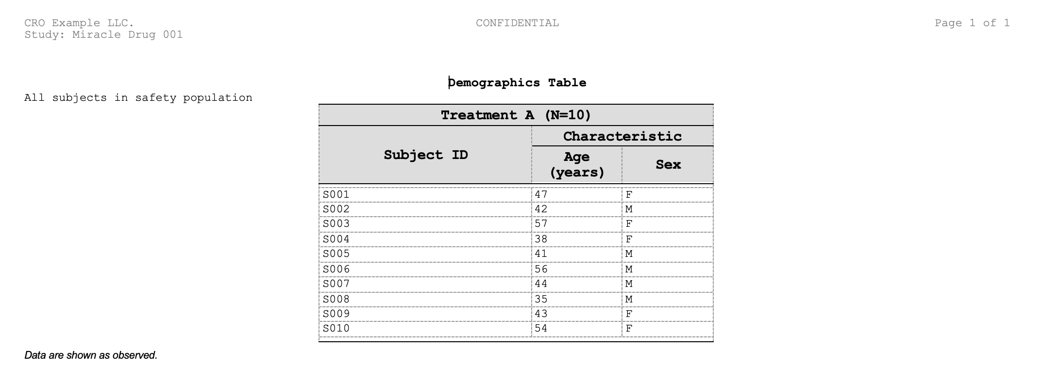

example complete demographics

Key gotchas and tips

Gotcha	Solution
*Calling s_ helpers outside add_style()**	Always use s_* inside `add_style()` — they validate context
define_cols() with mismatched parameter lengths	Length must be 1 (recycled) or match number of columns
Styles from f_combine() not consolidated	Call `create_report()` before `write_doc()`
Multiple add_header() calls stack	Each call appends a new header level; use `level =` to replace a specific level
Figure file not found	`create_figure()` errors immediately if the path is unreadable at call time — check the file exists and the path is right before saving
create_text() does not accept data	`create_text()` takes no arguments — add content via `add_body_text()`
Overlapping stubs at same stubOrder	Error; use different `stubOrder` or non-overlapping column sets

RStudio Addins

ksTFL ships with five RStudio Addins (available from the Addins drop-down in the RStudio toolbar). They provide interactive shortcuts for tasks that would otherwise require remembering function names or switching to the console.

Styles Editor

Launches a Shiny application for creating and editing style templates interactively. You can load any bundled template from tfl_list_templates(), modify fonts, borders, spacing, and colours in a WYSIWYG editor, then download the result as a JSON file ready for use with set_page_style() or write_doc(). This is especially useful when you need to fine-tune a template visually rather than writing s_font() / s_paragraph() / s_table_style() calls by hand.

Requires the shiny package.

# Equivalent programmatic call:
run_styles_editor()

Replay Reports

Opens a Shiny application for selecting, reordering, and combining previously saved reports into a single DOCX document. You point the app at one or more meta-data folders (produced by save_report() or write_doc()), drag-and-drop reports into the desired order, optionally enable a table of contents, and render the combined output — all without writing any R code.

Requires shiny, sortable, and shinyFiles packages.

# Equivalent programmatic call:
run_replay_app()

# Pre-populate a meta folder:
run_replay_app(meta_dir = "./output/meta")

TFL Spec Preview (Selection)

Evaluates the currently selected code in the source editor and, if the result is a TFL_spec, renders an HTML preview in the RStudio Viewer pane. This lets you highlight a pipeline expression (e.g., create_table(...) |> add_title(...)) and instantly see what the spec looks like — a quick visual check without saving or rendering to DOCX.

# Equivalent programmatic calls:
tfl_spec_preview_selection()   # preview of the editor selection
tfl_spec_preview_prompt()      # preview by object name (prompt)
view_tfl_spec(spec)            # preview a spec object directly

TFL Spec Preview (by name)

Same HTML preview, but instead of evaluating selected text the addin prompts you for the name of a TFL_spec object that already exists in .GlobalEnv. Handy when the spec was built interactively in the console and you want to preview it without re-selecting code.

Style Atoms Catalog

Prints all built-in style atoms to the console with colour-coded categories (font decoration, font family, font size, text colour, highlight, alignment, indentation, spacing, borders, backgrounds, row height, and more). Each atom is a short name you can reference directly in add_style() or define_cols() via f_combine(). Running this catalog helps you discover what is available without consulting documentation.

# Equivalent programmatic call:
tfl_style_atoms_catalog()
# — or —
tfl_print_style_atoms()

Next steps

You now understand ksTFL’s core workflow. Next steps:

Run the quick example above with your own data
Explore Reporting Examples for detailed patterns
Skim FAQ when something behaves unexpectedly — short answers, no detour required
Read Styling Guide for advanced styling
Read Advanced StyleRows for conditional formatting
Check function docs: ?create_table, ?define_cols, ?add_style, ?write_doc, ?list_reports

Resources

Function reference: ?ksTFL (package overview) or ?create_table, ?define_cols, etc.
Reporting Examples: Detailed working examples with explanations
Styling Guide: Comprehensive style reference
GitHub: ksTFL repository

Quick reference table

Task	Function	Notes
Create table spec	`create_table(data, cols = ...)`	Auto-detects columns, types, widths
Create figure spec	`create_figure(plot_or_path, dpi = 300L)`	File path or ggplot2 object; default device `cairo` (Word-safe paths-only SVG)
Create text spec	`create_text()`	For narrative content only
Set document properties	`set_document(spec, ...)`	Content width/placement, hasData, footnotePlace, isContinues, per-spec figure sizing (figureWidth/Height/Device/ScaleMode), docTemplate
Customize columns	`define_cols(spec, cols, ...)`	Use `c()` for multiple columns
Define styles	`add_style(spec, id = "name", ...)`	Use `s_font()`, `s_paragraph()`, `s_table_style()`
Add spanning header	`add_span_header(spec, cols, label, ...)`	Supports tidyselect; multi-level headers
Add titles/content	`add_title()`, `add_footnote()`, `add_body_text()`	Layer document content
Add page headers/footers	`add_header()`, `add_footer()`	3 parts: left/center/right
Conditional row actions	`compute_cols(spec, cond, ...)`	Use `c_style()`, `c_merge()`, `c_addrow()`, `c_glue()`, `c_clear()`, `c_pageBreak()`
Set page style	`set_page_style(spec, page = p_page(...))`	Configure page size, orientation, margins
Page settings helper	`p_page(size, orientation, margins)`	`"A4"`/`"A3"`/`"Letter"`/`"Legal"`/`"Executive"`, margins via `p_margins()`
List templates	`tfl_list_templates()`	Shows all bundled template names
Discover style atoms	`tfl_print_style_atoms()`	Prints all built-in style atoms grouped by category
Font status	`tfl_font_status()`, `tfl_rescan_fonts()`	Check or re-run font discovery
Combine specs	`create_report(spec1, spec2, ...)` or a named list	Consolidates styles, assigns order, finalizes compute_cols
Save + render (one step)	`write_doc(report, name, ...)`	Recommended: saves JSON + renders DOCX
Save only	`save_report(report, ...)`	Writes JSON + data files for manual rendering
Render from JSON	`replay_report(spec_json, meta_dir, output_path, overrideTemplate = NULL)`	C++ renderer: JSON → styled DOCX
Set session defaults	`tfl_set_options(...)`	Inherited by new specs in session
Check options	`tfl_get_options()`, `tfl_get_option(name)`	View current session settings
Reset options	`tfl_reset_options()`	Back to package defaults

ksTFL Development Team

2026-10-03

Introduction

How to use this guide

General workflow

High-level pipeline

Anatomy of a TFL spec

Quick 5-minute example

Step 1: Create a TFL_spec

Table spec (from data frame)

Figure spec (from image file)

Text spec (narrative content)

Step 2: Customize columns (define_cols)

Single column

Batch update (multiple columns with single values)

Per-column customization

Step 3: Define styles (add_style)

Step 4: Add spanning headers (span headers)

Step 5: Add titles, footnotes, headers, footers

Step 5b: Page layout and templates

Page size, orientation, and margins

Document templates

Step 6: Apply conditional row actions (compute_cols)

Step 7: Combine specs into a report

Passing a named list of specs

Step 8: Save and Render

Option A: One step with write_doc() (recommended)

Option B: Two steps with save_report() + replay_report()

Step 9: JSON metadata — what it is and why you might need it

What is the metadata folder?

Why use a persistent metaPath?

Managing metadata files

Recommended production setup

Understanding auto-generated values

Column widths (auto-calculation)

Data references (dataRef)

Session-wide defaults with tfl_set_options()

Complete example: From data to document

Key gotchas and tips

RStudio Addins

Styles Editor

Replay Reports

TFL Spec Preview (Selection)

TFL Spec Preview (by name)

Style Atoms Catalog

Next steps

Resources

Quick reference table

Option A: One step with `write_doc()` (recommended)

Option B: Two steps with `save_report()` + `replay_report()`

Session-wide defaults with `tfl_set_options()`