Condition Helpers: The Small Verbs Behind compute_cols()

ksTFL Development Team

2026-10-03

Why these helpers exist

compute_cols() is the workhorse of ksTFL formatting: you hand it a condition and one or more actions (c_style(), c_addrow(), c_glue(), …), and every row matching the condition gets treated. The obvious conditions are easy — AVAL > 12, TRTARM == "Treatment A". But most of what makes a clinical table read well is not about individual values. It is about position: this is where a new SOC block starts, this is the last row of the headache run, this is a subtotal line, this should look striped.

Plain column comparisons cannot express position. You could bolt it on with dplyr — mutate(is_first = !duplicated(SOC)), a helper column, another one for the zebra flag, and hide them all — and then your “flat analyst frame” quietly grows a tail of tags whose only purpose is to describe layout. ksTFL takes the other route: a handful of small functions that answer positional questions directly against the table data, inside the condition itself.

There are seven of them, and they split into three families:

Family	Helpers	Question they answer
Absolute	firstRow(), lastRow()	Is this the first / last row of the whole table?
Periodic	everyNth(n), rowNumber()	What number is this row? Does it fall on a beat?
Run-based	firstOf(...), lastOf(...), firstOfBlock(col, n, offset)	Where does a run of equal values begin and end?

One idea holds the whole third family together, and it is worth stating up front because it is the single most common source of surprise:

firstOf() / lastOf() / firstOfBlock() work on runs of contiguous equal values (run-length encoding), not on distinct values. In a frame sorted A, A, B, B, A, the function firstOf(GROUP) is TRUE on rows 1, 3 and 5 — the second block of As is a new run, so it gets a new “first”.

This is a feature, not a wart: ksTFL’s rendering contract is “the package paints your rows in the order you give them”. You arrange() the analyst frame upstream into exactly the reading order you want, and the run helpers then become a natural description of that order — “the first row of this visible block” — with no bookkeeping at render time. If your data really is grouped, sorted, and contiguous (and in clinical tables it almost always is), run semantics and “group” semantics coincide. When they don’t, the FAQ entry “Why does firstOf() mark more rows than I expected?” is the place to start.

All seven helpers are usable only inside the cond argument of compute_cols() (they are not exported to the global namespace), and they always look at the raw data, never at display text that earlier actions have already glued or cleared. Keep those two fences in mind and everything below falls into place.

Absolute markers: firstRow() and lastRow()

The simplest pair. They mark exactly one row each — the top and the bottom of the table — and they are the cleanest way to hang structural formatting: the booktabs-style rule under the header, the closing rule after the last result.

A treatment-emergent AE table with zebra banding on the odd rows (everyNth(2) marks rows 1, 3, 5, …) and heavy rules at the two absolute boundaries:

spec <- create_table(ae_by_pt) |>
  add_title("Table 1. Treatment-emergent adverse events by preferred term.") |>
  define_cols(SOC, label = "System organ class", colWidth = "24%") |>
  define_cols(PT,  label = "Preferred term",     colWidth = "22%") |>
  define_cols(c(TRTA, TRTNT, TOTAL),
              label = c("Treatment A<br>(N = 421)", "Treatment B<br>(N = 415)",
                        "Total<br>(N = 836)"),
              valueStyleRef = "ac", colWidth = "14%") |>
  # banding: everyNth(2) is TRUE on rows 1, 3, 5, 7 ...
  compute_cols(everyNth(2), c_style(everything(), styleRef = "bg_gray")) |>
  # structure: one rule under the header, one under the very last row
  compute_cols(firstRow(), c_style(everything(), styleRef = "bt")) |>
  compute_cols(lastRow(),  c_style(everything(), styleRef = "bb"))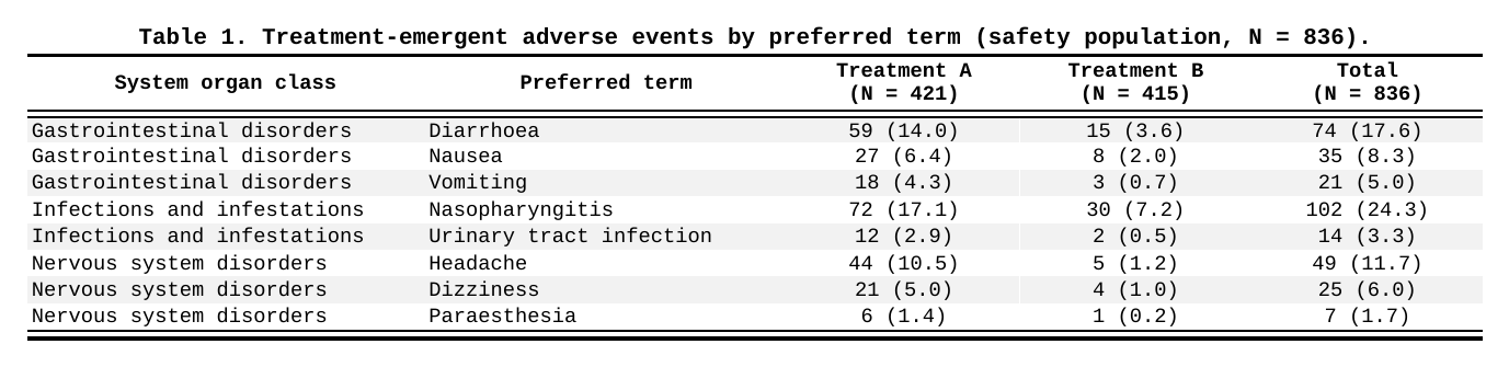

Zebra banding from everyNth() with bt/bb rules from firstRow()/lastRow()

Notice how the three rules read like a caption: band the odd rows, rule the top, rule the bottom. Three separate compute_cols() calls, each doing one visually distinct thing — which is exactly how you want to be able to edit them six months from now.

The same pair works whenever you need a boundary that is absolute rather than value-driven — a lab table where the first measurement row should be separated from the header no matter what the data says. Just remember that the marker is one row: if a table is paginated (isPaging), firstRow() still fires only on the true first row of the data, not on the first row of each page.

Run boundaries: firstOf() and lastOf()

The core pair. firstOf(col) is TRUE at the first row of every run of equal values in col; lastOf(col) mirrors it at the end of the run. Multiple columns are allowed — firstOf(A, B) marks runs of the pair, which is a handy way to say “this combination is new” without touching the data.

The most natural use is grouping structure without group columns. An AE incidence table where every SOC block should open and close with a thin rule:

spec <- create_table(ae_incidence) |>
  define_cols(SOC, label = "System organ class", colWidth = "30%") |>
  define_cols(PT,  label = "Preferred term",     colWidth = "26%") |>
  define_cols(INC, label = "Incidence<br>(%)", valueStyleRef = "ac", colWidth = "12%") |>
  define_cols(SEV, label = "Worst severity", valueStyleRef = "ac", colWidth = "16%") |>
  # a run of identical SOC starts here -> open the block
  compute_cols(firstOf(SOC), c_style(everything(), styleRef = "bt_th")) |>
  # ...and ends here -> close it
  compute_cols(lastOf(SOC),  c_style(everything(), styleRef = "bb_th"))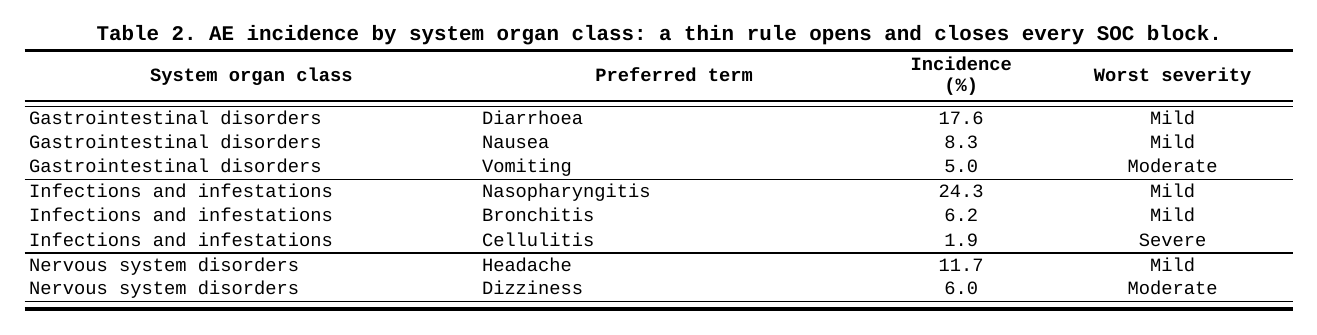

Thin top and bottom rules mark each SOC block via firstOf()/lastOf()

The repeated SOC text is still visually noisy here — two more lines fix it. This is the classic dedupe idiom: negate firstOf() and blank what it protects.

spec <- spec |>
  compute_cols(!firstOf(SOC), c_clear(SOC))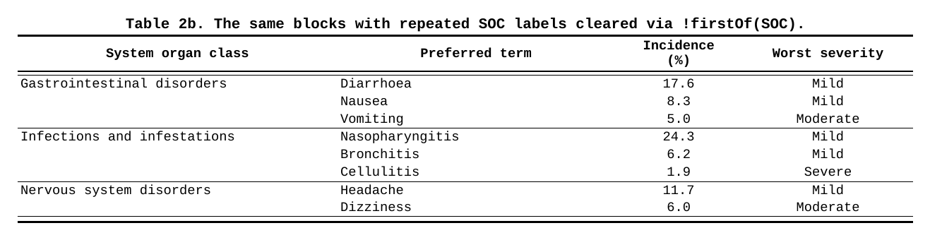

Repeated SOC labels cleared, blocks still ruled

A demographic table shows the multi-column variant properly, where two different notions of “is this row new?” live in two adjacent columns: age group changes slowly, treatment changes twice per age group. Blanking each label against its own run key gives the stepped reader’s-eye layout:

spec <- create_table(demog) |>
  define_cols(c(AGEGR1, TRTARM), label = c("Age group", "Treatment"), colWidth = "18%") |>
  define_cols(STAT, label = "Statistic", colWidth = "14%") |>
  define_cols(c(V1, V2), label = c("Visit 1<br>(Day 1)", "Visit 2<br>(Week 12)"),
              valueStyleRef = "ac", colWidth = "14%") |>
  # the age label lives only at the top of its own run
  compute_cols(!firstOf(AGEGR1), c_clear(AGEGR1)) |>
  # the treatment label re-appears at every new (age x treatment) combination
  compute_cols(!firstOf(AGEGR1, TRTARM), c_clear(TRTARM))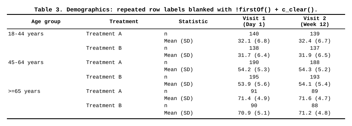

Demographics: AGEGR1 deduped per age group, TRTARM per age x treatment run

Why did Treatment A re-appear for the 45-64 group even though it is the same arm? Because firstOf(AGEGR1, TRTARM) describes a pair-run, and the run started over when the age group changed. One condition, no helper columns.

lastOf() earns its keep at the other end of the run — closing rules (above), subtotal insertion (later), and anywhere you must act “after the group is done” rather than “before it starts”.

Beat and number: everyNth() and rowNumber()

everyNth(n) is a tiny convenience: TRUE every n rows counting from row 1 (n = 2 marks rows 1, 3, 5 …). Two things to know. First, it counts rows, not groups or records — with grouped data a “zebra” built from everyNth(2) stripes the table, which is usually what you want, but does not respect block edges; if you need banding within each block only, combine with the run helpers (see the combination section). Second, when you want the other phase of the stripe, there is no everyNth(2, offset = 1) — you write the arithmetic yourself, and that is where rowNumber() comes in.

rowNumber() returns the row index (1-based) and composes in ordinary expressions: comparisons, modulo, ranges.

# even-row banding: the complement of everyNth(2)
compute_cols(rowNumber() %% 2 == 0, c_style(everything(), styleRef = "bg_gray"))

# "the first five rows are the top-5 AEs" -- a position rule
compute_cols(rowNumber() <= 5, c_style(PT, styleRef = "b"))

# "everything except the boundary rows" -- a range
compute_cols(rowNumber() > 1 & rowNumber() < 12, c_style(PARAM, styleRef = "ind1"))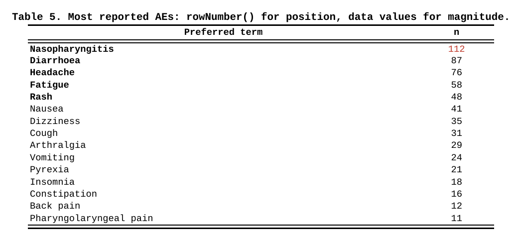

Most-reported AEs: top five PTs bold by rowNumber(), high counts by value

A position rule (rowNumber() <= 5) and a value rule (N >= 100) live comfortably side by side — this table shows both: the first five rows are bold because they are the top five, and 112 is red because it crosses a threshold. Pre-sorting the frame is what makes the position rule meaningful; the helpers then simply read the layout you arranged.

Periodic runs: firstOfBlock()

firstOfBlock(col, n = 1, offset = 0) is firstOf() with a metronome: it marks the first row of every n-th run of col — counting runs of equal values, skipping the first block, and starting after offset blocks. The mental model is “give me a beat that respects my blocks, not my rows”.

A compact AE table where you want breathing room between pairs of SOC blocks rather than between every one of them:

spec <- create_table(ae_compact) |>
  define_cols(SOC, label = "System organ class", colWidth = "34%") |>
  define_cols(PT,  label = "Preferred term",     colWidth = "30%") |>
  define_cols(ALL, label = "Any AE<br>(n (%))", valueStyleRef = "ac", colWidth = "16%") |>
  # first row of blocks 3, 5, ... gets an inserted spacer row above it
  compute_cols(firstOfBlock(SOC, n = 2), c_addrow(pos = "above"))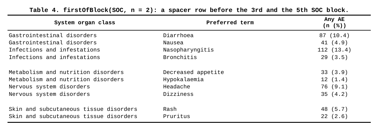

firstOfBlock(SOC, n = 2): empty spacer before the 3rd and 5th SOC block

The counting rule is the part to pin down: with five SOC blocks, firstOfBlock(SOC, n = 2) fires inside blocks 3 and 5. The first block never fires (nothing to separate it from), and every second block after that does. offset rotates the beat: offset = -1 moves it to the even blocks (2 and 4 — use it when the first gap should already be visible), offset = 1 pushes it one block further (4 and 6). Think of it as “skip offset extra blocks before the first marked one” and the three cases line up.

A typical honest use is a “block every other group” layout on long PK or lab tables, where grouping rows into visual pairs of visits or periods is cheaper than restructuring the data.

Combinations: where the helpers earn their keep

Individually the helpers are one-liners. Together with the actions they cover most of what a real table needs from conditional formatting, without a single tag column. The five combinations below are the ones that show up in production code over and over.

1. Footnote markers once per group: firstOf() + c_glue()

A PT reported at several grades should carry the footnote marker a exactly once, at its first appearance — and the repeated PT rows usually blank their label anyway. firstOf(PT) does the run work; c_glue() writes the marker:

spec <- create_table(ae_by_grade) |>
  define_cols(c(SOC, PT, GRADE), label = c("SOC", "PT", "Grade"), colWidth = "18%") |>
  define_cols(N, label = "n", valueStyleRef = "ac", colWidth = "8%") |>
  compute_cols(firstOf(PT),  c_glue(PT, "after", text = "<sup>a</sup>")) |>
  compute_cols(!firstOf(PT), c_clear(PT)) |>
  add_footnote("<sup>a</sup>PTs reported in more than one grade.")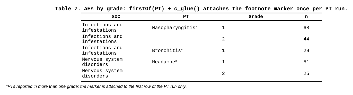

Superscript marker glued at firstOf(PT); repeated PT rows blanked

Inline markup (<sup>, <i>, …) is parsed inside glue text, so the marker renders as a real superscript. Note the pair firstOf / !firstOf on the same column — the positive marks where to glue, the negated one clears the rest; two honest halves of one layout rule.

2. Block headers from a hidden column: firstOf() + c_addrow()

The signature ksTFL idiom for sectioned tables. The analyst frame keeps SOC as a plain column; you hide it and let its first-row boundary become a real header row:

spec <- create_table(ae_blocks) |>
  define_cols(SOC, label = "SOC", isVisible = FALSE) |>
  define_cols(PT,  label = "Preferred term", colWidth = "40%") |>
  define_cols(c(TRTA, TRTNT, TOTAL),
              label = c("Treatment A<br>(N = 421)", "Treatment B<br>(N = 415)",
                        "Total<br>(N = 836)"),
              valueStyleRef = "ac", colWidth = "13%") |>
  compute_cols(firstOf(SOC),
               c_addrow(pos = "above", value_from = SOC, styleRef = "grp_hdr"))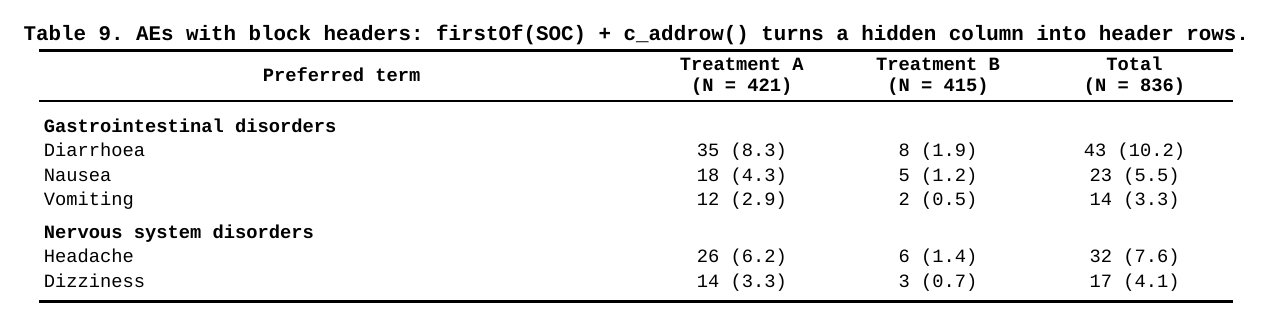

Generated header rows: firstOf(SOC) + c_addrow(value_from = SOC)

value_from = SOC copies the raw value into the synthetic row, and the styleRef belongs to the added row itself — later blocks will not repaint it. The price of admission: an added row is a single full-width cell, which is great for headers and no good for subtotals with per-column numbers. For those, see combination 3.

3. Subtotals assembled from the data: lastOf() + c_glue() + c_style()

Subtotal numbers belong to the data — the analyst computes them and appends a total row per block (a run member with an empty PT). Then lastOf(SOC) marks exactly those rows, because the subtotal extends its block’s run, and glue writes the label straight onto the still-present SOC value:

spec <- create_table(ae_subtotals) |>
  define_cols(SOC, label = "System organ class", colWidth = "26%") |>
  define_cols(PT,  label = "Preferred term",     colWidth = "24%", missings = "") |>
  define_cols(c(TRTA, TRTNT, TOTAL),
              label = c("Treatment A<br>(N = 421)", "Treatment B<br>(N = 415)",
                        "Total<br>(N = 836)"),
              valueStyleRef = "ac", colWidth = "13%") |>
  # keep SOC text at block top; subtotal rows (empty PT) keep theirs untouched
  compute_cols(!firstOf(SOC) & !is.na(PT), c_clear(SOC)) |>
  # the subtotal IS the last row of the run: prepend the label, bold, close
  compute_cols(lastOf(SOC),
    c_glue(SOC, "before", text = "Subtotal: "),
    c_style(everything(), styleRef = f_combine("b", "bb")))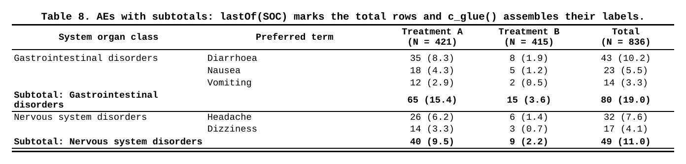

Subtotal rows marked by lastOf(SOC), labelled by c_glue, closed by a rule

Two subtleties worth naming. The first compute_cols() deliberately excludes the subtotal rows from clearing — !is.na(PT) — because the next block’s c_glue() decorates the text visible at action time, and on those rows the visible SOC is the label ingredient. The row’s own run membership still comes from the raw data: conditions read original values, c_clear() only blanks the painting. When the numbers must live in their columns (not in a synthetic full-width row), the frame holds them and the helpers merely point at them.

4. Gaps between blocks, but never at the edge: lastOf() + !lastRow()

Plain lastOf(SOC) + c_addrow(below) adds a gap after every block including the final one — a stray empty row before your footnotes. Compose the boundary helpers to express “between, not after”:

spec <- spec |>
  compute_cols(lastOf(SOC) & !lastRow(), c_addrow(pos = "below")) |>
  compute_cols(firstOf(SOC), c_style(SOC, styleRef = "b"))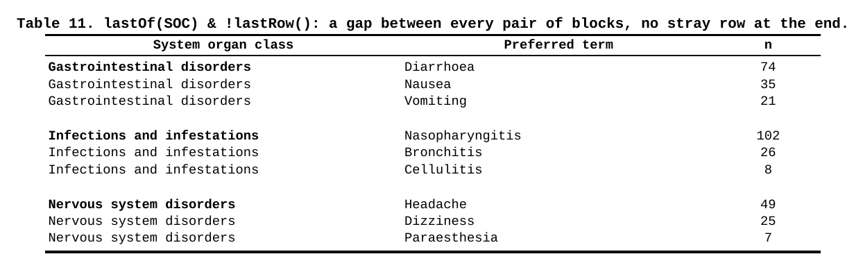

Spacer rows between SOC blocks; none after the last one

One run helper for the block edge, one absolute helper for the table edge, intersected in plain R logic. There is no dedicated “gap between groups” verb — the point of the design is that you do not need one.

5. Page breaks on block boundaries: firstOf() + rowNumber() + c_pageBreak()

Long safety exhibits often demand “one SOC per page”. The break belongs on the run start, minus the first row of the table — an absolute marker guarding the value boundary:

spec <- create_table(ae_socs) |>
  define_cols(SOC, label = "System organ class", colWidth = "34%") |>
  define_cols(PT,  label = "Preferred term",     colWidth = "30%") |>
  define_cols(N,   label = "n", valueStyleRef = "ac", colWidth = "10%") |>
  compute_cols(firstOf(SOC) & rowNumber() > 1, c_pageBreak())

Block one ends, block two starts a fresh page with a repeated header

Without the rowNumber() > 1 guard the renderer receives a page break on the very first row and you get a blank lead page — the same trick works with firstOfBlock() for “every second block on a new page”. The header row repeats on the new page by default, so each block arrives with its own context.

All of them at once

A production safety summary: hidden SECT column generates bold section headers (firstOf + c_addrow), every section but the last closes with a rule (lastOf + !lastRow), and the Total arm is bolded by plain value logic side-by-side with the run conditions:

spec <- create_table(safety_summary) |>
  define_cols(SECT, label = "Parameter", isVisible = FALSE) |>
  define_cols(TRTARM, label = "Treatment", colWidth = "30%") |>
  define_cols(c(N, EVT), label = c("n", "Events<br>(n (%))"), valueStyleRef = "ac",
              colWidth = "20%") |>
  compute_cols(firstOf(SECT),
               c_addrow(pos = "above", value_from = SECT, styleRef = "grp_hdr")) |>
  compute_cols(lastOf(SECT) & !lastRow(), c_style(everything(), styleRef = "bb")) |>
  compute_cols(TRTARM == "Total", c_style(c(TRTARM, N, EVT), styleRef = "b"))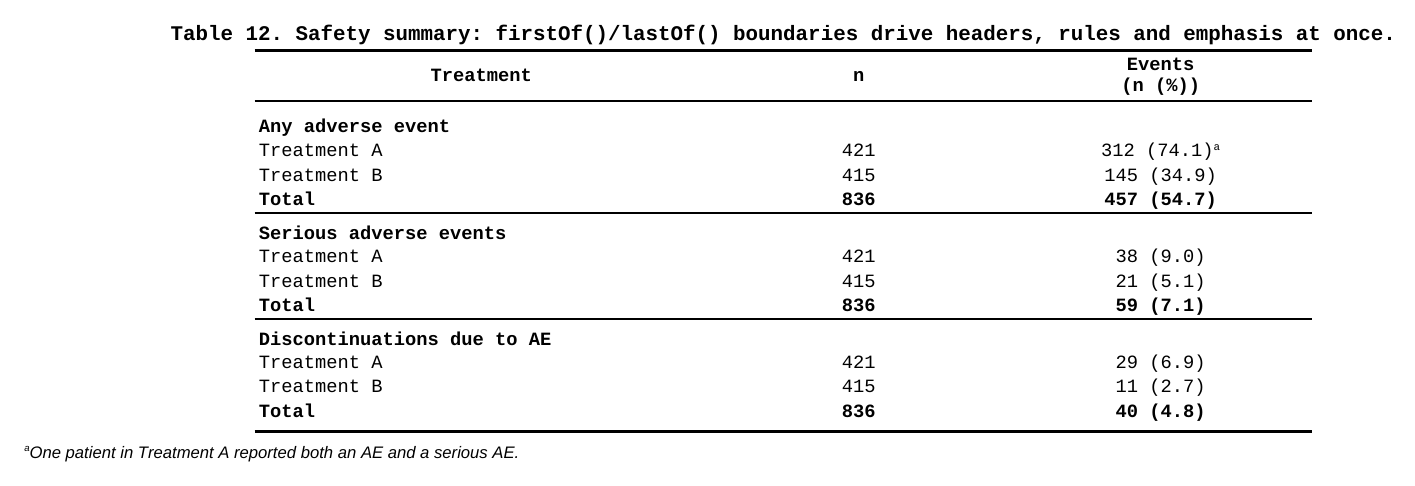

Section headers, closing rules and bold totals from three composed conditions

Three compute_cols() calls, one per visual feature — and the entire table is described in terms a reviewer can verify against the spec document line by line. No tag columns in the data, no post-processing pass, no template surgery.

Honest edges

Things to know before your first surprise:

• Run, not unique. All of firstOf / lastOf / firstOfBlock count contiguous runs. Non-sorted data with re-appearing values will look “over-marked”. Sort upstream — the renderer never will.
• Raw data for conditions, display state for glue sources. Conditions and value_from see the original values; c_clear() / c_glue() only change the painting — a later condition still matches a cleared cell’s underlying value. But c_glue(glue_col = ...) copies the cell’s text as it stands at action time: gluing a source that an earlier action cleared appends nothing.
• One added row = one full-width cell. Great for headers and spacers; put numeric subtotals in data rows instead (combination 3).
• value_from lands in the first cell of the synthetic row; there is no per-cell mapping across the added row.
• Paginating tables: firstRow() / lastRow() refer to absolute data positions, not per-page positions; everyNth() keeps counting across page breaks as well.
• NA in a condition is an error, not a skip — guard with !is.na(x) & when your frame can carry missing grouping values.

Reference table

Helper	Marks	Typical use
firstRow()	row 1	header rule, table-level emphasis
lastRow()	final row	closing rule, grand total styling
everyNth(n)	rows 1, n+1, 2n+1, …	zebra banding
rowNumber()	(returns indices)	ranges, modulo, top-N position rules
firstOf(cols)	start of each run	dedupe, block opening, headers, markers
lastOf(cols)	end of each run	closing rules, subtotal insertion
firstOfBlock(col, n, offset)	start of every n-th run	periodic block gaps

They are condition-only — available nowhere else in the DSL — and all of them are pure R against the frame you passed to create_table(). For action semantics and ordering (c_merge before c_clear before c_glue, style conflict resolution, addrow stacking), see Advanced StyleRows and Conditional Formatting; for the run-semantics gotcha in depth, see FAQ #13.