Advanced StyleRows and Conditional Formatting in ksTFL

Overview

This vignette covers conditional row formatting in ksTFL: compute_cols() and its six action functions — c_style(), c_merge(), c_addrow(), c_glue(), c_clear(), and c_pageBreak(). Rules are declared against the data and applied at render; no post-processing pass is needed.

Category and prerequisites

Prerequisites: complete Getting Started and basic compute_cols() familiarity. The focus here is row-level logic, helper functions, and composable actions that stay readable as rules grow.

Core Concept: Lazy Evaluation

compute_cols() uses lazy evaluation: it captures conditions and actions as quosures, stores them in the spec metadata, and evaluates them later during create_report().

Why Lazy Evaluation?

Deferred context: column selections and data references are resolved only after the report structure is complete.
Tidyselect support: helpers such as everything() and starts_with() stay available inside the action definitions.
Clean staging: you specify rules first and execute them later, which keeps the build pipeline easier to inspect.

Action Functions

`c_style()`: Conditional Styling

Apply style references to cells based on conditions:

library(ksTFL)

data <- data.frame(
  patient = sprintf("PAT-%03d", 1:20),
  age = c(23, 45, 67, 34, 89, 56, 42, 71, 38, 29,
          55, 66, 44, 52, 60, 48, 35, 70, 41, 58),
  response = sample(c("CR", "PR", "SD", "PD"), 20, replace = TRUE)
)

# Define styles first
spec <- create_table(data) |>
  add_style(id = "highlight_green", s_font(color = "#006400", bold = TRUE)) |>
  add_style(id = "highlight_red", s_font(color = "#8B0000", bold = TRUE))

# Apply conditional styling
spec <- spec |>
  compute_cols(
    response == "CR",
    c_style(response, styleRef = "highlight_green")
  ) |>
  compute_cols(
    response == "PD",
    c_style(response, styleRef = "highlight_red")
  )

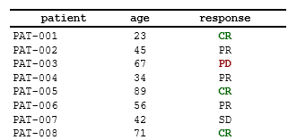
Result: The response cell shows green bold text on CR rows and red bold text on PD rows; other columns are untouched:

style conditional green red response

`c_merge()`: Conditional Cell Merging

Merge multiple columns into a single display cell:

data_groups <- data.frame(
  group = c("Treatment A", "Treatment A", "Treatment A",
            "Placebo", "Placebo"),
  visit = c("Week 0", "Week 4", "Week 8", "Week 0", "Week 4"),
  value = c(5.2, 6.1, 7.3, 4.8, 5.5)
)

spec <- create_table(data_groups) |>
  compute_cols(
    !firstOf(group),  # not the first row of each run of this group value
    c_merge(c(group, visit))
  )

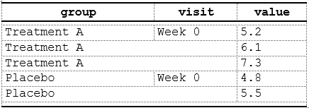
Result: When consecutive rows have the same group, their group and visit cells merge into one display cell showing the group value. The merged cell keeps the text of the leftmost column in the merged range (report column order), regardless of the order in which columns are listed in cols; the other columns’ values are not shown.

merge group visit cells

Note: The cols argument to c_merge() must resolve to at least two consecutive columns in the final report column order. Overlapping merges are not allowed: the second one is dropped with a warning.

`c_addrow()`: Conditional Row Insertion

Insert new rows based on data patterns:

spec <- create_table(data_groups) |>
  compute_cols(
    firstOf(group),  # First row of each group
    c_addrow(pos = "above")  # Insert an empty separator/header row above
  )

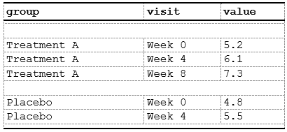
Result: The inserted row is one full-width cell: empty text without value_from, styled by styleRef — with a style it reads as a band or section header. To copy a single column’s value into the inserted row use value_from (see later examples). Use pos = "below" to insert after the matching row instead.

addrow separator above groups

`c_pageBreak()`: Conditional Page Break

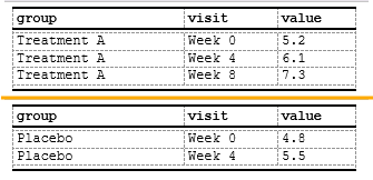
Insert a page break at the matching row. This is useful to force a new page when a logical grouping or large block ends.

spec <- create_table(data_groups) |>
  compute_cols(
    firstOf(group),  # Insert page break starting from first row of each group
    c_pageBreak()
  )

Result: The renderer will start a new page at rows matching the condition. Each break ends the current table segment and the next segment repeats the column-header row. A match on the very first data row changes nothing — that row already starts the page.

pagebreak at group start

Evaluation Context

The Data Environment

Conditions and actions are evaluated in spec$.metadata$data_env, which contains:

Data columns: Direct access to all columns (even invisible ones)
Helper functions: firstOf(), lastOf(), firstRow(), lastRow(), rowNumber(), everyNth(), firstOfBlock()
Embedded functions: Internal utilities for column access

Important: These helper functions are only available inside the cond argument of compute_cols(). They are not standalone exported functions — you cannot call them outside of compute_cols().

Style references passed to actions can also name built-in atoms (b, i, ar, indent_1, bg_mint, bt_th, …; full catalog via tfl_print_style_atoms() and in the Styling Guide); f_combine() merges several atoms into one reference.

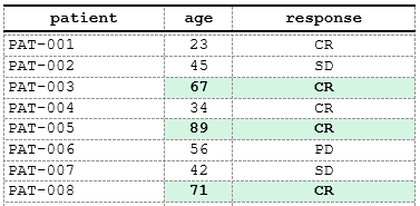
# You can reference any column directly in conditions
spec <- create_table(data) |>
  compute_cols(
    age > 60 & response %in% c("CR", "PR"),  # Multi-column condition
    c_style(c(age, response), styleRef = f_combine('b', 'bg_mint'))
  )

style multi column conditional

Available Helper Functions

The following helpers are available exclusively inside compute_cols() conditions:

firstOf(...): Logical vector TRUE at the first row of each RUN of equal values in the specified columns (run-length semantics). Sort the data upstream so each logical group is contiguous — a value that re-appears later starts a new run and matches again.
lastOf(...): The same, TRUE at the last row of each run.
firstRow(): Logical vector TRUE only at first row
lastRow(): Logical vector TRUE only at last row
rowNumber(): Integer vector of row numbers (1-based)
everyNth(n): Logical vector TRUE at every nth row starting from row 1 (so everyNth(2) marks odd rows 1, 3, 5, …; use rowNumber() %% 2 == 0 for the even rows)
firstOfBlock(col, n = 1, offset = 0): TRUE at the first row of every n-th RUN of col values, excluding the first run — n = 1 marks the start of runs 2, 3, 4, …; n = 2 marks runs 3, 5, … Same sort precondition as firstOf().

# Highlight first and last rows using helper functions
spec <- create_table(data) |>
  add_style(id = "border_emphasis",
            s_font(bold = TRUE),
            s_table_style(borders = s_borders(top = s_border(width = "2pt"),
                                              bottom = s_border(width = "2pt")))) |>
  compute_cols(
    firstRow() | lastRow(),
    c_style(everything(), styleRef = "border_emphasis")
  )

# Use firstOf/lastOf for value-based boundaries
spec <- create_table(data_groups) |>
  add_style(id = "group_boundary", s_font(bold = TRUE)) |>
  compute_cols(
    firstOf(group) | lastOf(group),
    c_style(group, styleRef = "group_boundary")
  )

# Use everyNth for alternating patterns
spec <- create_table(data) |>
  add_style(id = "gray_bg", s_table_style(background_color = "#F5F5F5")) |>
  compute_cols(
    everyNth(2),  # marks odd rows: 1, 3, 5, ...
    c_style(everything(), styleRef = "gray_bg")
  )

Advanced `c_style()` Patterns

Multiple Column Styling

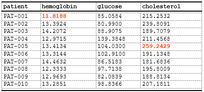
Use tidyselect to style multiple columns at once:

data_lab <- data.frame(
  patient = sprintf("PAT-%03d", 1:10),
  hemoglobin = rnorm(10, 13.5, 1.5),
  glucose = rnorm(10, 95, 15),
  cholesterol = rnorm(10, 200, 30)
)

spec <- create_table(data_lab) |>
  add_style(id = "out_of_range", s_font(color = "#FF4500", bold = TRUE)) |>
  compute_cols(
    hemoglobin < 12 | hemoglobin > 16,
    c_style(hemoglobin, styleRef = "out_of_range")
  ) |>
  compute_cols(
    glucose < 70 | glucose > 140,
    c_style(glucose, styleRef = "out_of_range")
  ) |>
  compute_cols(
    cholesterol > 240,
    c_style(cholesterol, styleRef = "out_of_range")
  )

style out of range highlight

Conditional Styling with Complex Logic

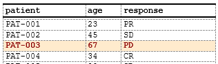
Combine multiple conditions:

spec <- create_table(data) |>
  add_style(id = "critical_senior",
            s_font(color = "#8B0000", bold = TRUE),
            s_table_style(background_color = "#FFEBCD")) |>
  compute_cols(
    age >= 60 & response == "PD",
    c_style(c(patient, age, response), styleRef = "critical_senior")
  )

style critical senior age

Row-Level Styling

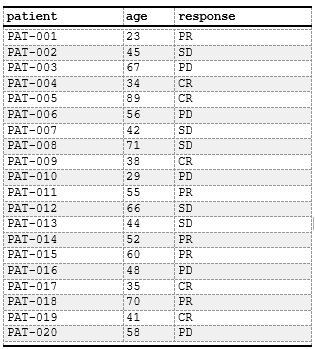
Style entire rows by targeting all columns:

spec <- create_table(data) |>
  add_style(id = "alternate_row",
            s_table_style(background_color = "#F0F0F0")) |>
  compute_cols(
    rowNumber() %% 2 == 0,  # Even rows
    c_style(everything(), styleRef = "alternate_row")
  )

style alternating row colors

Advanced `c_merge()` Patterns

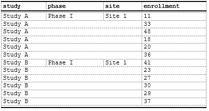
Multi-Column Grouping Merges

Merge across multiple grouping levels:

data_nested <- data.frame(
  study = rep(c("Study A", "Study B"), each = 6),
  phase = rep(c("Phase I", "Phase II", "Phase III"), 4),
  site = rep(c("Site 1", "Site 2", "Site 1", "Site 2"), 3),
  enrollment = sample(10:50, 12)
)

spec <- create_table(data_nested) |>
  # Merge study column for consecutive same-study rows
  compute_cols(
    !firstOf(study),
    c_merge(c(study, phase, site))
  ) |>
  # Merge phase column within same study
  compute_cols(
    !firstOf(study, phase),
    c_merge(c(phase, site))
  )

merge multi column grouping

Merging with Styling

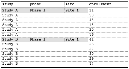
Combine merging with conditional styles:

spec <- create_table(data_nested) |>
  add_style(id = "merged_header",
            s_font(bold = TRUE),
            s_table_style(background_color = "#E0E0E0")) |>
  compute_cols(
    !firstOf(study),
    c_merge(c(study, phase, site))
  ) |>
  compute_cols(
    firstOf(study),  # First row of group
    c_style(study, styleRef = "merged_header")
  )

merge with styling

Advanced `c_addrow()` Patterns

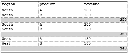
Summary Rows

Insert calculated summary rows:

data_sales <- data.frame(
  region = c("North", "North", "South", "South", "West", "West"),
  product = rep(c("A", "B"), 3),
  revenue = c(100, 150, 200, 120, 180, 160),
  total =   c(250, 250, 320, 320, 340, 340)
)

spec <- create_table(data_sales) |>
  add_style(id = "summary_row",
            s_font(bold = TRUE),
            s_table_style(background_color = "#D3D3D3")) |>
  # we do not need the `total` column itself - set to invisible
  define_cols(total, isVisible = F) |> 
  compute_cols(
    lastOf(region),  # Last row of each region
    # Insert subtotal row
    c_addrow(pos = "below", 
             value_from = total, #value from total column
             styleRef = f_combine("summary_row", 'ar'))  
  )

addrow summary subtotals

Header Rows

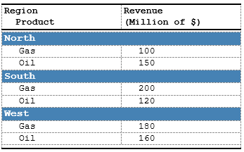
Insert section (group) headers to make a stub:


data_sales <- data.frame(
  region = c("North", "North", "South", "South", "West", "West"),
  product = rep(c("Gas", "Oil"), 3),
  revenue = c(100, 150, 200, 120, 180, 160)
)

spec <- create_table(data_sales) |>
  # Custom style just for fun
  add_style(id = "section_header",
            s_font(bold = TRUE, font_size = "10pt", color = '#FFFFFF'),
            s_table_style(background_color = "#4682B4")) |>
  # Hide the `region` column as we want to use its value as heading
  define_cols(region, isVisible = F) |>
  # Add column labels:
  define_cols(
    c(product, revenue),
    label = c('Region<br>  Product', 'Revenue<br>(Million of $)'),
    # Use embedded indent style to indent the `product` value in a column
    valueStyleRef = c('indent_1', NA) # NA here means we are not using any style for `revenue`
  ) |>
  # Use `c_addrow` to add a line with the value from `region` column
  compute_cols(
    firstOf(region),  # First row of each new region
    c_addrow(pos = "above", 
             value_from = region,
             styleRef = "section_header")
  )

addrow header from column

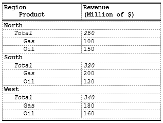
More complex example with two-level indents:


data_sales <- data.frame(
  region = c("North", "North", "North", "South", "South", "South", "West", "West", "West"), 
  product = rep(c("Total","Gas", "Oil"), 3),
  revenue = c(250, 100, 150, 320, 200, 120, 340, 180, 160)
)


spec <- create_table(data_sales) |>
  # Hide the `region` column as we want to use its value as heading
  define_cols(region, isVisible = F) |>
  # Add column labels:
  define_cols(
    c(product, revenue),
    label = c('Region<br>    Product', 'Revenue<br>(Million of $)')
  ) |>
  # Use `c_addrow` to add a line with the value from `region` column
  compute_cols(
    firstOf(region),  # First row of each new region
    c_addrow(pos = "above",  
             value_from = region,
             styleRef = 'b')
  ) |>
  # the `Total` value will be indented 0.5cm
  compute_cols(
    product == 'Total',
    c_style(product, f_combine('i', 'indent_1')),
    c_style(revenue, 'i')
  ) |>
  # Other values ('Gas', 'Oil') will be indented by 1cm
  compute_cols(
    product != 'Total',
    c_style(product, 'indent_2') 
  )

As a result we are getting two-level stub:

addrow two level stub indent

`c_glue()`: Append or Prepend Text to Cell Values

c_glue() concatenates a literal string or a data column value to the display text of matching cells — useful for appending units, prefixing markers, or building composite labels without creating extra columns.

Parameters:

cols: columns to modify (tidyselect)
position: "before" or "after" — where to attach the text
glue_col: unquoted name of a data column whose value to attach
text: a literal string (single value) to attach
separator: string inserted between original value and the glued text (default "")

Provide exactly one of glue_col / text. If both appear in a compute_cols() call, the parser warns and keeps glue_col, ignoring text.

Glue lands on the raw cell text: a cell suppressed by dedupe or merged as a non-leader renders blank and the glued part is skipped — target the merge leader. cols must match visible report columns; glue_col may reference a hidden one.

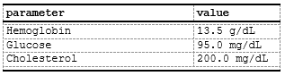
data_units <- data.frame(
  parameter = c("Hemoglobin", "Glucose", "Cholesterol"),
  value     = c(13.5,          95.0,      200.0),
  unit      = c("g/dL",        "mg/dL",   "mg/dL")
)

spec <- create_table(data_units) |>
  # Hide the unit column — use it only as a glue source
  define_cols(unit, isVisible = FALSE) |>
  # Append unit to value: "13.5" → "13.5 g/dL"
  compute_cols(
    !is.na(value),
    c_glue(value, position = "after", glue_col = unit, separator = " ")
  )

glue append units

c_glue() is fully compatible with c_style() and c_merge() in the same compute_cols() call.

`c_clear()`: Blank Cell Content in Matching Rows

c_clear() renders specified cells as empty (blank) in matching rows without removing the column or affecting layout. Useful for conditional deduplication, when the dedupe parameter of define_cols() is not enough.

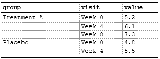
data_groups <- data.frame(
  group  = c("Treatment A", "Treatment A", "Treatment A", "Placebo", "Placebo"),
  visit  = c("Week 0", "Week 4", "Week 8", "Week 0", "Week 4"),
  value  = c(5.2, 6.1, 7.3, 4.8, 5.5)
)

spec <- create_table(data_groups) |>
  # Show group label only on first row of each group; blank it on the rest
  compute_cols(
    !firstOf(group),
    c_clear(group)
  )

clear blank cells

Note: c_clear() only affects the rendered display text. The underlying data value is still available for conditions in other compute_cols() calls. Actions run in arrival order, so c_clear() before c_glue() in the same call turns the glue into a full cell replacement, while c_glue() before c_clear() erases the glued result.

Combining Actions Together

Chain multiple compute_cols() calls and c_* actions to build a fully formatted table:

data_sales <- data.frame(
  region = c("North", "North", "North", 
             "South", "South", "South", 
             "West", "West", "West"),
  product = rep(c("Oil", "Gas", "TOTAL"), 3),
  revenue = c(100, 150, 250, 200, 120, 320, 180, 160, 340)
)

spec <- create_table(data_sales) |>
  add_style(id = "section_header",
            s_font(bold = TRUE, font_size = "11pt", color = '#FFFFFF'),
            s_table_style(background_color = "#4682B4")) |>
  # Make Region invisible, since we want to make it as header row
  define_cols(region, isVisible = F) |>
  # Define column labels
  define_cols(c(product, revenue), label = c('Product', 'Revenue<br>(Million of $)')) |>
  # Make a header row from the `region` value
  compute_cols(
    firstOf(region),  # First row of each new region
    c_addrow(pos = "above", 
             value_from = region,
             styleRef = "section_header")
  ) |> 
  # Create a summary row for `Total` value
  # Note here how a consecutive calls to `c_*` atomic functions produce final result
  compute_cols(
    product == 'TOTAL',
    # merge `product` and `revenue` to a single column (the value became value from `product`)
    c_merge(c(product, revenue), styleRef = f_combine('b','i','bt_th','ar')), 
    # clear the value, since we want to rebuild it:
    c_clear(product),
    # take the value of `region` into the merged cell...
    c_glue(product, 'after', glue_col = region),
    # then the word 'total: ' ...
    c_glue(product, 'after', text = ' total: '),
    # and finally the `revenue` value to complete the string
    c_glue(product, 'after', glue_col = revenue)
  )

Here we can see how a simple planar data frame:

data simple planar dataframe

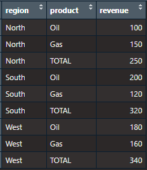
become a production ready table:
result production ready table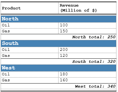

Performance Tips

One condition block per rule

Every compute_cols() block adds one condition/action group to the spec and one resolution pass at create_report(). There is no case_when construct inside conditions — group rules under a shared condition when they apply together, and keep style lookups cheap by reusing ids:

# Three rules over the same column (idiomatic):
spec <- create_table(data) |>
  add_style(id = "young",  s_font(color = "#008000")) |>
  add_style(id = "middle", s_font(color = "#0000FF")) |>
  add_style(id = "senior", s_font(color = "#FF0000")) |>
  compute_cols(age < 30, c_style(age, styleRef = "young")) |>
  compute_cols(age >= 30 & age < 60, c_style(age, styleRef = "middle")) |>
  compute_cols(age >= 60, c_style(age, styleRef = "senior"))

# When the same action set applies to several ranges, merge the ranges
# into ONE condition with `|`:
spec <- create_table(data) |>
  add_style(id = "extreme", s_font(bold = TRUE)) |>
  compute_cols(age < 25 | age >= 65, c_style(age, styleRef = "extreme"))

Use Vectorized Conditions

Avoid row-by-row operations in custom functions:

# ❌ Slower (scalar logic):
spec <- create_table(data) |>
  add_style(id = "responder", s_font(bold = TRUE)) |>
  compute_cols(
    sapply(response, function(x) x %in% c("CR", "PR")),  # Row-by-row
    c_style(response, styleRef = "responder")
  )

# ✅ Faster (vectorized):
spec <- create_table(data) |>
  add_style(id = "responder", s_font(bold = TRUE)) |>
  compute_cols(
    response %in% c("CR", "PR"),  # Vectorized
    c_style(response, styleRef = "responder")
  )

Tighten Conditions, Do Not Split Tables

Conditions are evaluated vectorized, one pass per block over whole columns — there is no per-row cost to optimize. If only a few rows need styling, make the condition selective (e.g. age > 80), not the data: do not split one logical table across two specs for formatting reasons, because each spec becomes its own Word table in the report.

Style Consolidation

ksTFL automatically consolidates identical styles, but you can help by reusing style references:

# ✅ Define once, use many times:
spec <- create_table(data) |>
  add_style(id = "critical", s_font(color = "#FF0000", bold = TRUE)) |>
  compute_cols(age > 80, c_style(age, styleRef = "critical")) |>
  compute_cols(response == "PD", c_style(response, styleRef = "critical"))

# ❌ Avoid duplicate style definitions:
# (This creates two identical but separate styles)
spec <- create_table(data) |>
  add_style(id = "critical_age",      s_font(color = "#FF0000", bold = TRUE)) |>
  add_style(id = "critical_response", s_font(color = "#FF0000", bold = TRUE))

Debugging and Inspection

Viewing Captured Actions

Inspect what compute_cols() has stored:

spec <- create_table(data) |>
  compute_cols(
    age > 60,
    c_style(age, styleRef = "elderly")
  )

# Examine metadata (internal structure — read-only, may change between versions)
str(spec$.metadata$compute_cols)
# Shows the captured condition quosures and per-block action lists

Testing Conditions Manually

Test conditions on your data frame before adding to spec:

# Test your condition directly on the data before passing to compute_cols()
test_condition <- with(data, age > 60)
sum(test_condition)   # How many rows match?
data[test_condition, ]  # Which rows?

# Once confirmed, add to spec
spec <- spec |>
  compute_cols(age > 60, c_style(age, styleRef = "elderly"))

Incremental Building

Add compute_cols() one at a time and inspect results:

spec <- create_table(data)

# Add first action
spec <- spec |>
  compute_cols(age > 60, c_style(age, styleRef = "elderly"))
print(spec)  # Check structure

# Add second action
spec <- spec |>
  compute_cols(response == "CR", c_style(response, styleRef = "success"))
print(spec)  # Check again

Common Patterns Library

Pattern 1: Alternating Row Colors

spec <- create_table(data) |>
  add_style(id = "gray_bg", s_table_style(background_color = "#F5F5F5")) |>
  compute_cols(
    rowNumber() %% 2 == 0,
    c_style(everything(), styleRef = "gray_bg")
  )

Pattern 2: Group Separator Bands with Cell Merging

spec <- create_table(data_groups) |>
  add_style(id = "group_header",
            s_font(bold = TRUE, font_size = "11pt"),
            s_table_style(background_color = "#D0D0D0")) |>
  # Insert a styled band row above each new group
  compute_cols(
    firstOf(group),
    c_addrow(pos = "above", styleRef = "group_header")
  ) |>
  # Merge consecutive same-group cells
  compute_cols(
    !firstOf(group),
    c_merge(c(group, visit))
  )

Pattern 3: Conditional Highlighting with Thresholds

spec <- create_table(data_lab) |>
  add_style(id = "low",    s_font(color = "#0000FF")) |>
  add_style(id = "normal", s_font(color = "#008000")) |>
  add_style(id = "high",   s_font(color = "#FF0000")) |>
  compute_cols(
    hemoglobin < 12,
    c_style(hemoglobin, styleRef = "low")
  ) |>
  compute_cols(
    hemoglobin >= 12 & hemoglobin <= 16,
    c_style(hemoglobin, styleRef = "normal")
  ) |>
  compute_cols(
    hemoglobin > 16,
    c_style(hemoglobin, styleRef = "high")
  )

Pattern 4: Summary Rows with Totals

# The analyst frame carries a pre-computed per-region total in `total`
# (same value repeated on every row of the region).
data_totals <- data.frame(
  region  = rep(c("North", "South"), each = 2),
  product = rep(c("A", "B"), 2),
  revenue = c(100, 150, 200, 120),
  total   = c(250, 250, 320, 320)
)

spec <- create_table(data_totals) |>
  add_style(id = "total_row",
            s_font(bold = TRUE),
            s_table_style(background_color = "#FFD700")) |>
  define_cols(total, isVisible = FALSE) |>
  compute_cols(
    lastOf(region),  # Last row of each region
    # copy the region total into a full-width row below it
    c_addrow(pos = "below", value_from = total, styleRef = "total_row")
  )

Limitations and Workarounds

Limitation 1: Conditions must be row-wise

The condition expression must evaluate to a logical vector with exactly one element per data row, or a single logical scalar (recycled to all rows). Anything else errors at create_report():

# ❌ Wrong-length result: the condition may capture fine, but
#    create_report() aborts because it resolves lazily:
spec <- create_table(data) |>
  add_style(id = "above_average", s_font(italic = TRUE)) |>
  compute_cols(
    age > head(mean(age), 0),  # returns logical(0), not one value per row
    c_style(age, styleRef = "above_average")
  )
create_report(spec)  # aborts: condition must return a length-20 logical

Scalar-returning aggregates DO work — they are recycled across rows:

spec <- create_table(data) |>
  add_style(id = "above_average", s_font(italic = TRUE)) |>
  compute_cols(
    age > mean(age),   # scalar mean -> age > 29.5 for every row
    c_style(age, styleRef = "above_average")
  )

Still, the recommended idiom is precomputing helper columns upstream — it is explicit, cacheable, and lets invisible columns drive several rules at once:

data$age_above_avg <- data$age > mean(data$age)

spec <- create_table(data) |>
  define_cols(age_above_avg, isVisible = FALSE) |>
  compute_cols(
    age_above_avg,
    c_style(age, styleRef = "above_average")
  )

Limitation 2: No Nested `c_*()` Functions

You can’t nest action functions:

# ❌ This is invalid: actions are siblings, not expressions that can be
#    nested inside each other's arguments. (Aborts at create_report():
#    the nested c_merge() has no compute_cols() context when resolved.)
spec <- create_table(data) |>
  compute_cols(
    age > 60,
    c_style(age, styleRef = c_merge(c(patient, age)))  # Not allowed
  )
create_report(spec)

Workaround: Use separate compute_cols() calls:

spec <- create_table(data) |>
  compute_cols(age > 60, c_style(age, styleRef = "elderly")) |>
  compute_cols(age > 60, c_merge(c(patient, age)))

Limitation 3: Style References Must Exist

styleRef must reference a previously defined style:

# ❌ This will error at evaluation time (create_report validates all
#    referenced style ids):
spec <- create_table(data) |>
  compute_cols(age > 60, c_style(age, styleRef = "undefined_style"))
create_report(spec)

Workaround: Always define styles before using them:

spec <- create_table(data) |>
  add_style(id = "elderly", s_font(bold = TRUE)) |>  # Define first
  compute_cols(age > 60, c_style(age, styleRef = "elderly"))

Integration with Other ksTFL Features

Using with `define_cols()`

compute_cols() works alongside column definitions:

spec <- create_table(data) |>
  add_style(id = "elderly", s_font(bold = TRUE)) |>
  define_cols(age, type = "numeric", format = "0.0", colWidth = "15%") |>
  compute_cols(
    age > 65,
    c_style(age, styleRef = "elderly")
  )

Using with Invisible Columns

Reference invisible columns in conditions:

data$flag <- sample(c(TRUE, FALSE), nrow(data), replace = TRUE)

spec <- create_table(data) |>
  add_style(id = "flagged", s_font(color = "#B8860B", bold = TRUE)) |>
  define_cols(flag, isVisible = FALSE) |>  # Hide column
  compute_cols(
    flag == TRUE,  # But use it in condition
    c_style(response, styleRef = "flagged")
  )

Using in Multi-Spec Reports

Each spec can have independent compute_cols() logic:

spec1 <- create_table(data[1:10, ]) |>
  add_style(id = "elderly", s_font(bold = TRUE)) |>
  compute_cols(age > 60, c_style(age, styleRef = "elderly"))

spec2 <- create_table(data[11:20, ]) |>
  add_style(id = "success", s_font(bold = TRUE)) |>
  compute_cols(response == "CR", c_style(response, styleRef = "success"))

report <- create_report(spec1, spec2)

Best Practices

Define styles first: Use add_style() before compute_cols()
Test conditions incrementally: Add one compute_cols() at a time
Use meaningful style names: “elderly” is clearer than “style1”
Document complex logic: Add comments explaining condition rationale
Prefer vectorized operations: Avoid row-by-row functions where possible
Reuse styles: Define once, reference many times for consistency
Keep conditions simple: Complex logic is harder to debug
Use helper functions: firstOf(), lastOf(), firstRow(), lastRow() are more readable than complex comparisons

Summary

compute_cols(): Captures conditions and actions via lazy evaluation
c_style(): Apply conditional styling to cells
c_merge(): Merge cells across columns based on conditions
c_addrow(): Insert new rows dynamically (pos = "above" or "below")
c_glue(): Append or prepend a string or another column’s value to the display text of matching cells
c_pageBreak(): Insert a page break at the matching row
c_clear(): Blank the rendered display text of specified cells in matching rows (deduplication)
Evaluation context: condition-only helpers (firstOf(), lastOf(), firstRow(), lastRow(), rowNumber(), everyNth(), firstOfBlock()) resolved inside the spec data environment — not exported functions
Performance: Minimize calls, use vectorized operations, consolidate styles
Debugging: Inspect metadata, test conditions manually, build incrementally

For more information, see:

Getting Started — full pipeline overview and compute_cols() introduction
Styling Guide — styling fundamentals and built-in atoms
Reporting Examples — complete end-to-end workflows
Column Width Management — invisible columns for conditional logic

ksTFL Development Team

2026-10-03